

prophys#


Risk models you can differentiate
Write the geometry, the physics and the uncertainty of a problem as one Python model. prophys compiles it into a single JAX graph. You sample it, fit it to measurements and optimise a design with the same gradient, and every number comes back with its error bar.
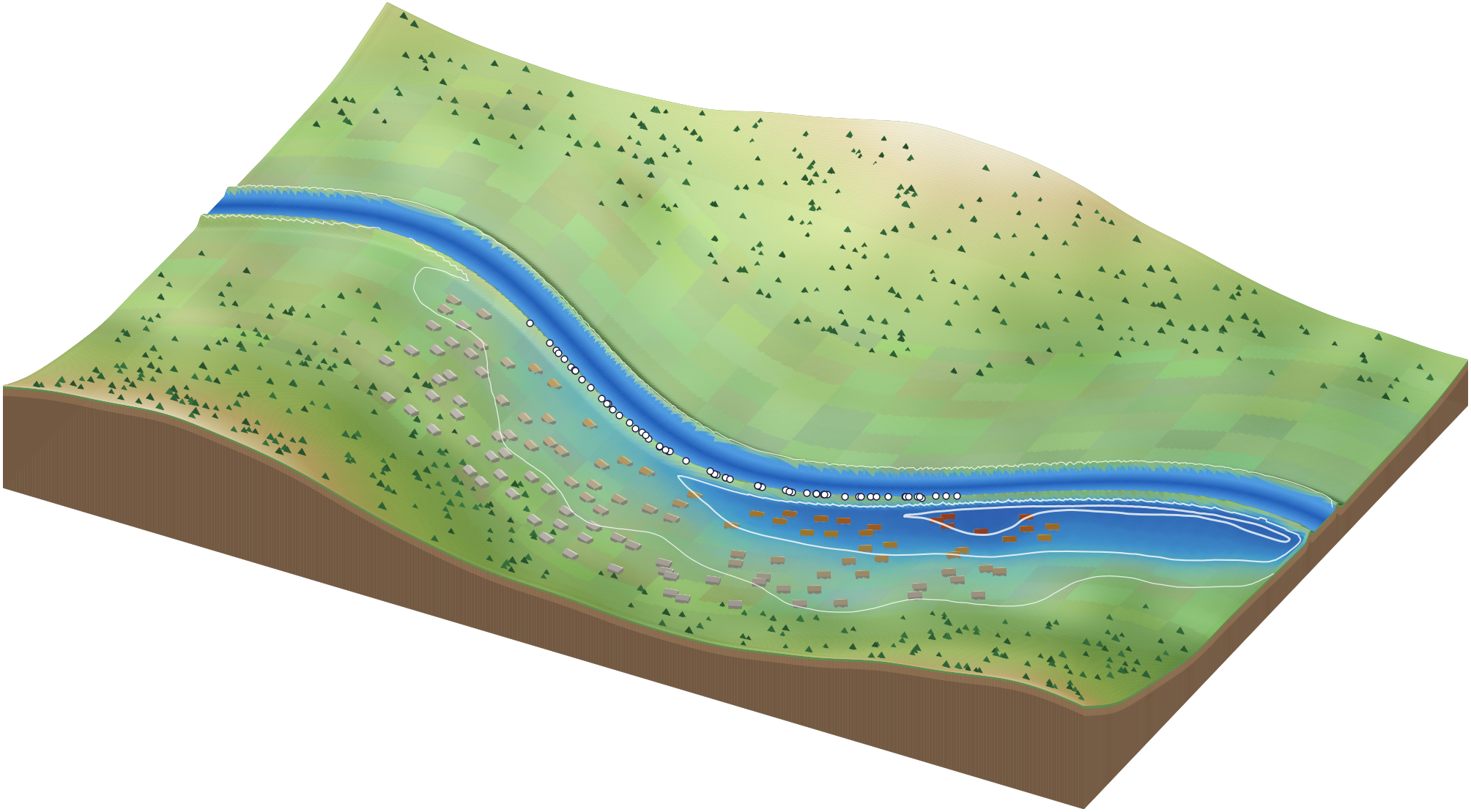
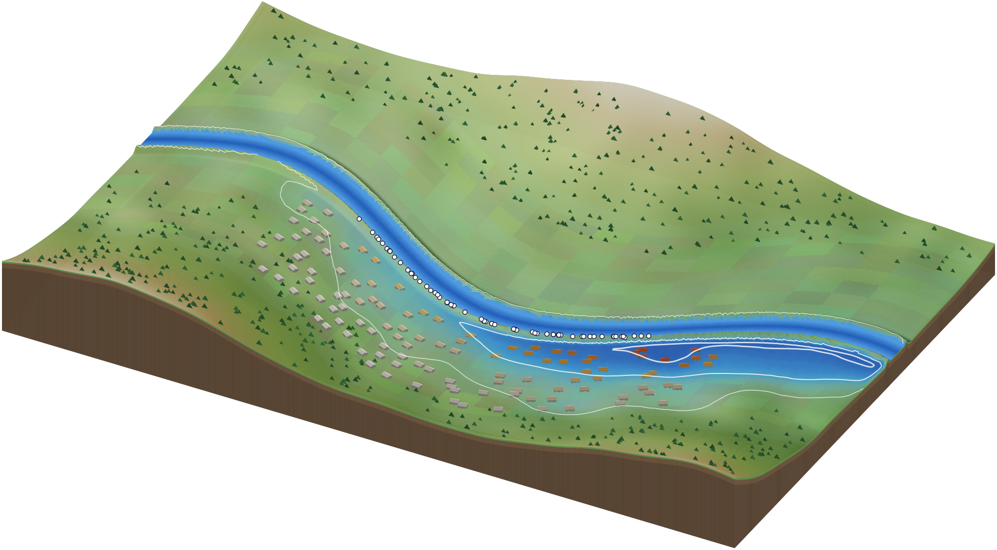
A levee breach at an uncertain place, 64 Monte Carlo runs of a shallow water model. Blue shows how likely each field floods, roofs turn from white to red with the chance that a house takes on more than 30 cm of water, dots mark the sampled breaches.
One graph
Geometry, physics, learned surrogates and probability distributions sit in the same compiled model. A pipeline route, a copula correlation and a network weight move in the same optimiser step.
Error bars on everything
Monte Carlo standard errors, parameter intervals, Sobol and Shapley attributions and predictive scores come with each run, together with a manifest of what produced it.
The same numerics on every device
Optimized native kernels run the numerics on CPU and GPU. On the tested GPUs, forward results match the CPU bit for bit. Learned surrogates train at TensorFlow speed and ship to a runtime that needs no Python.
prophys is proprietary software by RhineQC GmbH.
Learned surrogates in the graph#
A surrogate learns what nobody wrote down, a power curve from SCADA rows, a failure rate from incident records, the next state of a flow field. prophys pretrains it on its own data and then keeps training it inside the model, next to every physical parameter, with its uncertainty in every risk number. Physics you do know goes into the network as a physics layer and exports with it.
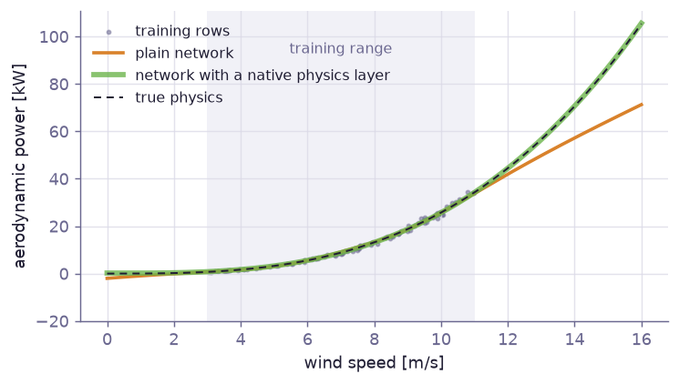
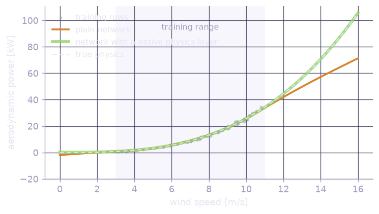
A cube law written as a prophys expression compiles into the network and keeps the fit right outside the training range.
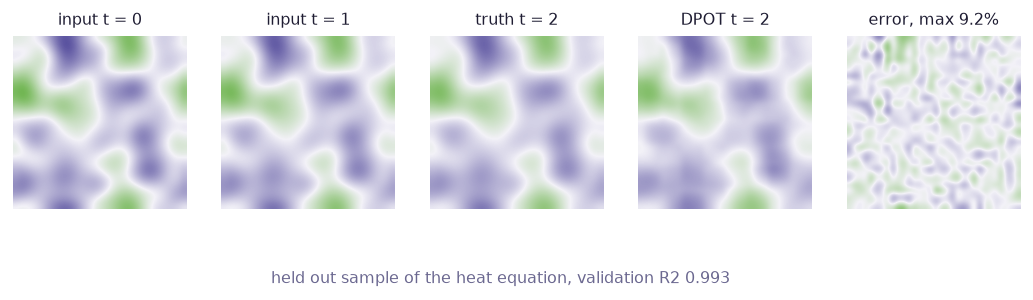
DPOT checkpoints convert by name, match PyTorch to round off and train faster than PyTorch on the CPU.
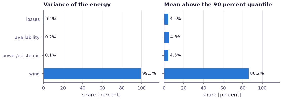
Shapley values of variance and CVaR through the whole model, and exact TreeSHAP for tree ensembles.
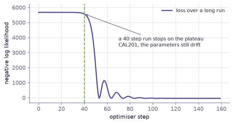
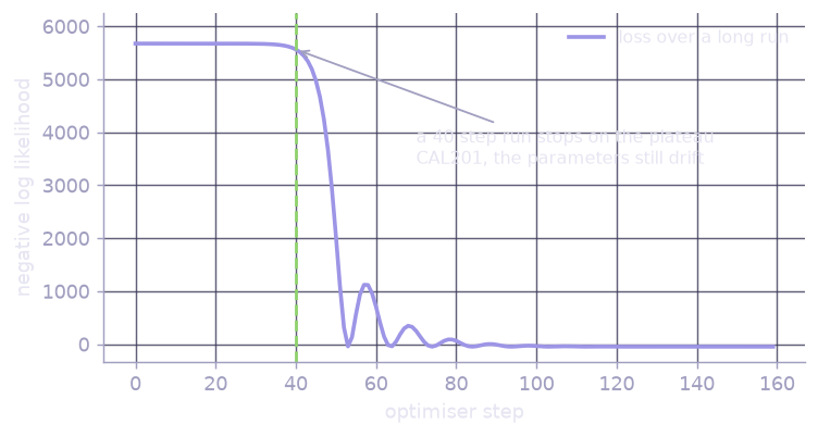
Coded diagnostics catch shape errors at build time and runs that stopped on a plateau before the loss dropped.
One toolkit, many domains#
The primitives that model a gas leak also model a grid cascade, a wind farm or a reinsurance layer. What carries over is the ability to calibrate and optimise geometry, physics and uncertainty together, whatever the domain.
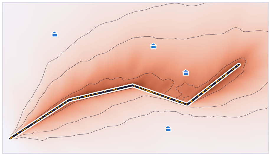
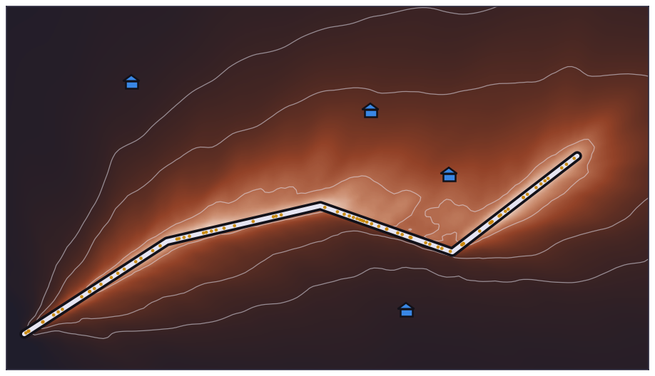
A Gaussian plume whose leak point is drawn anywhere along the route, wind as upstream random variables, exposure and its tail, a calibrated dose response and abatement optimised by gradient.
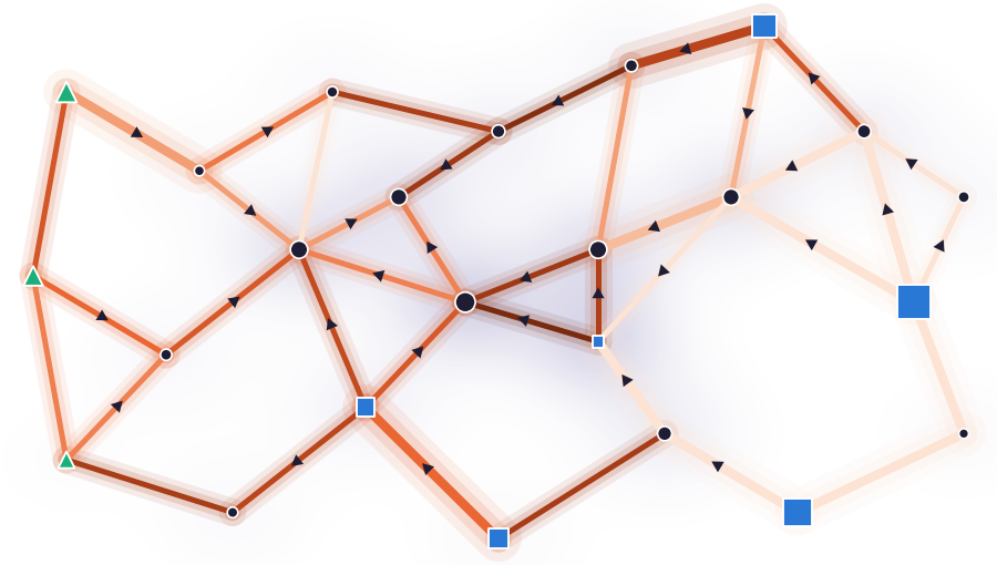
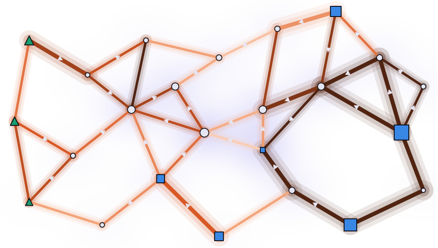
PTDF and LODF from the gradient of a DC power flow, overload cascades under uncertain wind and demand, and line upgrades optimised by gradient.
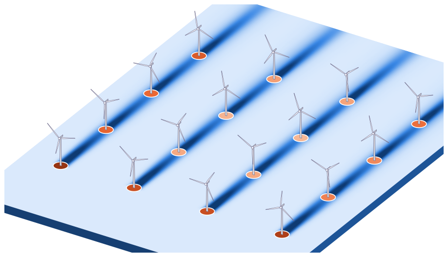
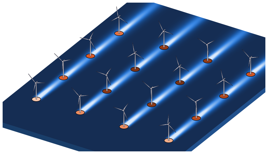
DirectionalMixture couples sector weights, circular spread and a
speed distribution per sector into a wind rose you can calibrate and
feed to siting or fatigue models.
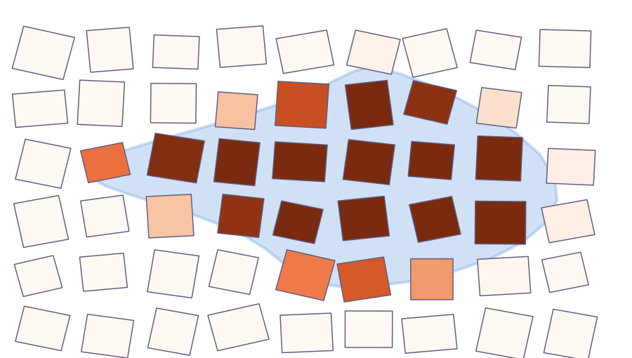
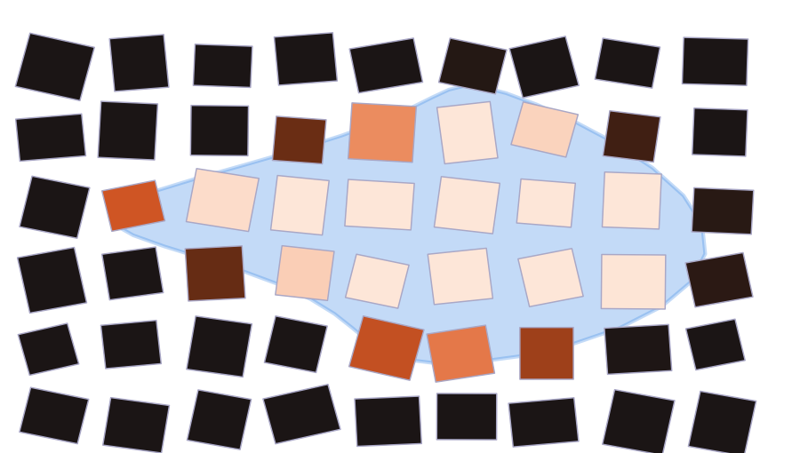
Terrain rasters and portfolio polygons with hazards coupled by a
GaussianCopula. Spatially correlated loss stays differentiable, so
pricing sensitivities come for free.
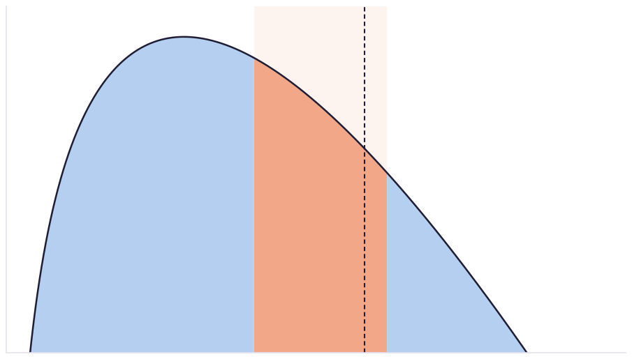
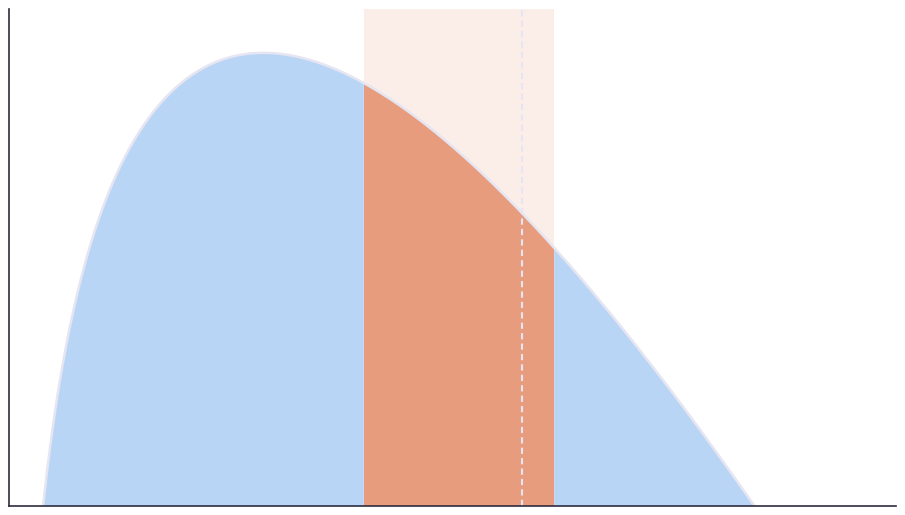
Heavy tailed severities with quantile() and cvar() on any
attribute, and attachment points tuned by gradient.
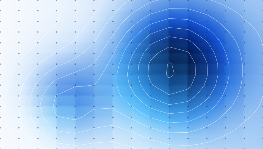

Solver output on a Mesh or a voxel Field3D becomes a
differentiable input, ready to calibrate against point measurements.
Guides#
Points, lines, polygons, polyhedra, fields, grids, networks and meshes.
Univariate, circular, multivariate, mixture and copula families.
Fit parameters to observations and optimise design variables.
Monte Carlo errors, parameter intervals and profile likelihoods.
Local derivatives, elasticities and Sobol decompositions.
WAIC, PSIS LOO, PIT, CRPS and posterior predictive checks.
NUTS over the compiled model through NumPyro.
CSV with non detects, wind roses, rasters and NetCDF, with units.
Model packages, surrogate blobs and the C runtime.
A first model#
Two houses, two turbines whose positions are parameters, a noise level that falls with distance and a Weibull acceptance drop that depends on it.
import prophys as prp
import jax.numpy as jnp

site = prp.Frame("site")
houses = prp.PointList(jnp.array([[0.0, 0.0], [200.0, 0.0]]), site)
turbines = prp.PointList(prp.Param("pos", shape=(2, 2), init=jnp.array([[80.0, 80.0], [150.0, 20.0]])), site)

distance = houses.closest_distance(turbines, mode="opt", tau=2.0)
level = prp.Param("base", init=100.0) - 20 * prp.log10(distance)

acceptance = prp.UncertainAttribute("acceptance_drop", prp.Weibull(scale=1.0 + level, concentration=prp.Param("k", init=2.0)))
model = prp.ProbabilityModel(acceptance)
compiled = model.compile(mode="opt")

print(compiled.expectation("acceptance_drop"))