Training & Design Optimization

Training & Design Optimization#

Both parameter training (fit distribution/model parameters to data) and design optimization (choose a design variable, e.g. a position or an abatement fraction, to minimize/maximize an objective) reduce to the same operation: gradient descent through the compiled graph via Optax. The only difference is what plays the role of “the parameter being optimized” and what plays “the objective.”

Three training entry points, from narrowest to widest scope:

Function	Scope
`fit_distribution()`	One standalone distribution (univariate or multivariate), no model needed
`calibrate()`	A compiled model, against observations of one attribute
`finetune()`	The entire model jointly, against observations of several attributes at once

Calibration (MLE / MAP)#

import prophys as prp

compiled = model.compile()
result = prp.calibrate(
    compiled,
    "acceptance_drop",       # attribute name
    observations,            # array of observed values
    n_steps=300,
    learning_rate=0.05,
)
print(result.params)         # fitted parameters, constrained space
print(result.final_loss)

Internally, calibrate() builds the negative log-likelihood (optionally plus a prior term for MAP) as a function of the model’s unconstrained parameters — the same space Param.forward maps back from — so Adam never has to worry about box constraints or positivity; those are enforced structurally by the parameterization itself.

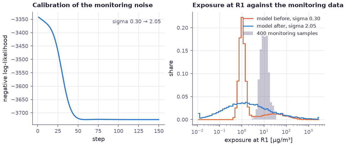
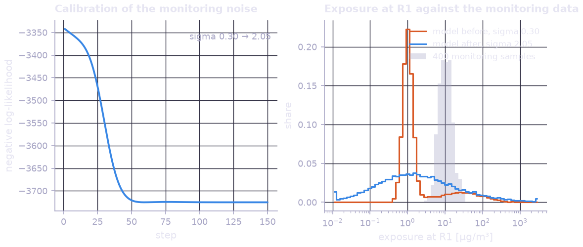
Calibration of the monitoring noise in the gas dispersion example

Calibration in the pipeline-leak example (:doc:`examples/gas_dispersion`). Left: the negative log-likelihood of 400 monitoring samples while the noise level is fitted. Right: the modelled exposure before and after, against the samples.

Freezing and selecting parameters#

Both calibrate() and finetune() accept trainable=[...] (whitelist) or frozen=[...] (blacklist) of parameter names. Frozen parameters keep their current values but still participate in the forward computation — the standard workflow for staged fitting (fit the physics first, then the noise model, then release everything for a final joint pass).

prp.calibrate(compiled, "complaints", records, trainable=["dose_k", "dose_x0"])
prp.finetune(compiled, all_observations, frozen=["emission_rate"])

Finetuning the entire model#

finetune() maximizes the joint likelihood over several attributes at once. Because attributes typically share upstream parameters (a common emission rate, a shared monitoring sigma, a copula correlation), joint fitting pools every observation’s information into every shared parameter — with per-attribute weights if some data sources are more trustworthy than others:

result = prp.finetune(
    compiled,
    {"exposure_res0": exposure_obs, "complaint_res0": complaint_records},
    weights={"complaint_res0": 2.0},
)

Fine tuning learned surrogates#

When a model contains pretrained surrogates (Learned Surrogates), finetune() anchors them to their pretraining with surrogate_feedback. The pretraining posterior (an exact Laplace posterior of the head and a diagonal Gauss Newton precision of every other weight) is raised to the power 1 / feedback and added to the loss:

fit = prp.finetune(model, observations,
                   surrogate_feedback=1.0,      # 0 cut, 1 joint, above 1 trust the outcome data more
                   surrogate_scope="head")      # or "all"
fit.surrogate_shift(power_curve)                 # shift per leaf in nats

With surrogate_scope="head" and no explicit trainable list, the physical parameters and the final linear layer of each surrogate (the leaves of tree ensembles) train and the rest stays at its pretrained weights. Calibration results report convergence findings in diagnostics and converged, see Diagnostics.

Learning distributions directly#

fit_distribution() trains the Param leaves of a standalone distribution — no model required, and multivariate data works the same way as univariate (the leading axis indexes observations):

# Univariate: recover Weibull parameters from samples
w = prp.Weibull(scale=prp.Param("scale", init=5.0, transform="softplus"),
               concentration=prp.Param("k", init=1.0, transform="softplus"))
prp.fit_distribution(w, wind_measurements)

# Multivariate: learn a full covariance via its Cholesky factor
mvn = prp.MultivariateGaussian(
    mean=prp.Param("mu", shape=(2,), init=jnp.zeros(2)),
    cholesky=prp.Param("L", shape=(2, 2), init=jnp.eye(2)),
)
prp.fit_distribution(mvn, paired_measurements)

# Mixtures: learn component weights (softmax-normalized logits)
mix = prp.Mixture([prp.Gaussian(0.0, 1.0), prp.Gaussian(10.0, 1.0)],
                 logits=prp.Param("logits", shape=(2,), init=jnp.zeros(2)))
prp.fit_distribution(mix, samples)

The Cholesky and copula parameterizations are chosen so any unconstrained gradient step yields a valid covariance/correlation — no projections, no clipping, no failed updates.

Design optimization#

result = prp.optimize(
    objective,               # a scalar Expr to minimize
    wrt=[turbine_positions],
    constraints=[min_spacing_violation],  # each must evaluate <= 0
    n_steps=200,
    learning_rate=1.0,
)
print(result.params["pos"])

Constraints are enforced via a quadratic penalty; per-parameter bounds don’t need a constraint at all, since a bounded Param already can’t leave its valid range under any gradient step.

If the objective references a RandomVariable (e.g. optimizing for a specific wind condition rather than marginalizing over it), bind it via extra_env:

result = prp.optimize(
    objective,
    wrt=[abatement_param],
    extra_env={"wind_speed": 6.0, "wind_direction": jnp.deg2rad(35.0)},
)

Using a compiled model in external JAX solvers#

A CompiledModel is a bundle of pure JAX functions — nothing about it is tied to prophys’ own Optax loops. Any quantity it produces (an expectation, a log-likelihood, a CVaR) can be closed over in an ordinary Python function of a parameter pytree and handed to any JAX-gradient-based solver; gradients flow through the native kernels exactly as they do inside prophys:

import jax

def objective(raw_params):
    # any scalar the model can produce; raw_params is unconstrained space
    return -compiled.log_prob("exposure", observations, params=raw_params).sum()

value_and_grad = jax.jit(jax.value_and_grad(objective))

# jaxopt
import jaxopt
result = jaxopt.LBFGS(fun=objective).run(compiled.default_params())

# optimistix
import optimistix as optx
sol = optx.minimise(lambda p, _: objective(p), optx.BFGS(rtol=1e-6, atol=1e-6),
                    compiled.default_params())

# scipy, via JAX-computed gradients
from scipy.optimize import minimize
import numpy as np
flat0 = np.asarray(compiled.default_params()["sigma"])
# ... flatten/unflatten with jax.flatten_util.ravel_pytree as usual

The same applies to symbolic expressions directly: expr.evaluate(env) is a pure function of env, so jax.grad(lambda v: expr.evaluate({"x": v})) works with any downstream solver, inside or outside jit.

Diagnostics#

finite_difference_check() compares jax.grad against central finite differences — useful whenever a Surrogate wraps hand-written physics, to catch a silent mismatch between the analytic and autodiff gradient. check_identifiability() is a cheap heuristic flag for “the loss was still improving meaningfully when optimization stopped.”

See also

Observations: Fitting against censored, interval or missing records rather than exact values.
Uncertainty & Error: Standard errors, confidence intervals and profile likelihoods for the parameters a fit returns.
Model Validation: Whether the fitted model is any good, and whether it beats another.
Posterior Inference: The full posterior rather than a point estimate.

prophys.engine.calibrate(compiled, attribute_name, observations, *, prior_neg_log_prob=None, init_params=None, trainable=None, frozen=None, n_steps=500, learning_rate=0.01, optimizer=None)[source]#

Fit the parameters of a compiled model to observations of one attribute.

Maximizes the total log likelihood of observations under the attribute attribute_name (maximum likelihood), or the log posterior when prior_neg_log_prob is given (maximum a posteriori), by gradient descent in unconstrained parameter space. Equivalent to finetune(compiled, {attribute_name: observations}, ...). Use finetune() to fit several attributes jointly.

Parameters:

compiled (CompiledModel) – The model, from ProbabilityModel.compile(). Compile with mode="opt" when geometry kernels need smooth gradients.
attribute_name (str) – The observed attribute.
observations (Any) – A one dimensional array of exact observations (one per row), or an Observations record carrying censored or missing values.
prior_neg_log_prob (Callable[[Mapping[str, Any]], Any] | None) – Optional f(constrained_params) -> scalar added to the loss, for a MAP fit.
init_params (Mapping[str, Any] | None) – Starting values by name in unconstrained space. Other parameters start at their declared init. Also sets the value frozen parameters are held at.
trainable (Iterable[str] | None) – Names or glob patterns ("power/*") of the only parameters to update. Takes precedence over frozen.
frozen (Iterable[str] | None) – Names or glob patterns of parameters to hold fixed.
n_steps (int) – Number of optimizer steps.
learning_rate (float) – Learning rate of the default Adam optimizer.
optimizer (GradientTransformation | None) – An Optax optimizer to use instead of Adam.

Returns:

A CalibrationResult. Convergence problems are reported as warnings and in its diagnostics.

Raises:

KeyError – If attribute_name or a trainable or frozen name is unknown.
ValueError – If no parameter is left to train.

Return type:

CalibrationResult

Example

>>> compiled = model.compile(mode="opt")
>>> fit = calibrate(compiled, "concentration", measured, n_steps=300)
>>> fit.params["emission_rate"]

prophys.engine.finetune(compiled, observations, *, weights=None, prior_neg_log_prob=None, init_params=None, trainable=None, frozen=None, n_steps=500, learning_rate=0.01, optimizer=None, surrogate_feedback=None, surrogate_scope='head')[source]#

Jointly fit a compiled model against observations of several attributes.

The loss is the (optionally weighted) sum of every observed attribute’s negative log likelihood, plus an optional prior term. Because attributes typically share upstream parameters (a common emission rate, a shared noise sigma, a copula correlation), joint fitting propagates every observation’s information into every shared parameter: this is the “train the entire model” entry point, and it trains learned surrogates in the graph together with the physical parameters.

Parameters:

compiled (CompiledModel) – The model, from ProbabilityModel.compile().
observations (Mapping[str, Any]) – Attribute name to a one dimensional array of exact observations or an Observations record (censored or missing values).
weights (Mapping[str, float] | None) – Optional weight of each attribute’s log likelihood by name (default 1).
prior_neg_log_prob (Callable[[Mapping[str, Any]], Any] | None) – Optional f(constrained_params) -> scalar added to the loss, for a MAP fit.
init_params (Mapping[str, Any] | None) – Starting values by name in unconstrained space. Other parameters start at their declared init. Frozen parameters named here are held at the given value.
trainable (Iterable[str] | None) – Names or glob patterns ("power/*") of the only parameters to update. Takes precedence over frozen.
frozen (Iterable[str] | None) – Names or glob patterns of parameters to hold fixed. Ignored when trainable is given, and also when surrogate_feedback is set, which then picks trainable itself.
n_steps (int) – Number of optimizer steps.
learning_rate (float) – Learning rate of the default Adam optimizer.
optimizer (GradientTransformation | None) – An Optax optimizer to use instead of Adam.
surrogate_feedback (float | Mapping[str, float] | None) – Anchors every pretrained surrogate to its pretraining posterior raised to the power 1 / feedback. Zero adds no anchor and, unless trainable is given, holds the surrogate at its pretrained weights (cut feedback). One is full joint estimation, values in between let the outcome data move the surrogate less. A float applies to every surrogate, a mapping sets it per surrogate name and surrogates it leaves out get one. None (default) adds no anchor.
surrogate_scope (str) – Which surrogate leaves train when surrogate_feedback is set and trainable is not. "head" for the final linear layer (or the leaf values of a tree ensemble), "all" for every leaf. Parameters outside any surrogate always train.

Returns:

A CalibrationResult. With surrogate_feedback its surrogate_priors holds the pretrained priors of every surrogate.

Raises:

KeyError – If an attribute or a trainable or frozen name is unknown.
ValueError – If no parameter is left to train. A ProphysError (NN101), itself a ValueError, if surrogate_feedback is set and surrogate_scope is neither "head" nor "all".

Return type:

CalibrationResult

Example

>>> fit = finetune(compiled, {"energy": metered, "load": strain},
...                surrogate_feedback=1.0)

prophys.engine.fit_distribution(distribution, data, *, prior_neg_log_prob=None, init_params=None, n_steps=500, learning_rate=0.01, optimizer=None)[source]#

Fit the Param leaves of a standalone distribution to data by maximum likelihood.

No ProbabilityModel is required. Works for univariate data (a one dimensional array of scalar observations) and multivariate data alike. The leading axis of data indexes observations and each row is passed to log_prob unchanged, so a MultivariateGaussian with a learnable Cholesky factor, a Mixture with learnable logits, or any distribution whose parameters are Param expressions is fitted the same way.

Parameters:

distribution – A distribution built with Param parameters.
data (Any) – Observations, shape (n,) or (n, d).
prior_neg_log_prob (Callable[[Mapping[str, Any]], Any] | None) – Optional f(constrained_params) -> scalar added to the loss, for a MAP fit.
init_params (Mapping[str, Any] | None) – Starting values by name in unconstrained space. Other parameters start at their declared init.
n_steps (int) – Number of optimizer steps.
learning_rate (float) – Learning rate of the default Adam optimizer.
optimizer (GradientTransformation | None) – An Optax optimizer to use instead of Adam.

Returns:

A CalibrationResult with the fitted parameters.

Raises:

ValueError – If the distribution has no Param leaves.

Return type:

CalibrationResult

Example

>>> from prophys import Param, fit_distribution
>>> from prophys.distributions import Gaussian
>>> d = Gaussian(mean=Param("mu", init=0.0),
...              sigma=Param("sigma", init=1.0, transform="softplus"))
>>> fit = fit_distribution(d, data, n_steps=1000, learning_rate=0.05)
>>> fit.params["mu"], fit.params["sigma"]

prophys.engine.optimize(objective, *, wrt, init_params=None, constraints=(), penalty_weight=1000.0, n_steps=500, learning_rate=0.01, optimizer=None, extra_env=None)[source]#

Minimize a scalar objective over design parameters, with inequality constraints.

Runs gradient descent on the Param leaves listed in wrt, in their unconstrained space. Each constraint is an Expr that must evaluate to <= 0. Violations are penalized quadratically, adding penalty_weight * sum(max(c, 0) ** 2) to the objective. Param.forward already maps bounded parameters through a sigmoid or softplus, so box constraints on single parameters need no penalty. Only constraints that couple parameters (for example a minimum spacing between turbines) belong in constraints.

Unlike CompiledModel.expectation(), design optimization conditions on a scenario rather than marginalizing over it. extra_env binds any leaves other than Param that the objective or constraints reference, such as a RandomVariable fixed at the median wind condition.

Parameters:

objective (Expr) – Scalar expression to minimize.
wrt (Sequence[Any]) – The Param instances to optimize.
init_params (Mapping[str, Any] | None) – Starting values by parameter name, in unconstrained space. Every name must be in wrt. Parameters not given start at their declared init.
constraints (Sequence[Expr]) – Expressions required to be <= 0 at the optimum.
penalty_weight (float) – Weight of the quadratic constraint penalty.
n_steps (int) – Number of optimizer steps.
learning_rate (float) – Learning rate of the default Adam optimizer.
optimizer (GradientTransformation | None) – An Optax optimizer to use instead of Adam. learning_rate is then ignored.
extra_env (Mapping[str, Any] | None) – Fixed values by name for leaves that are not Param.

Returns:

An OptimizationResult with the optimized parameters in constrained space and the loss history.

Return type:

OptimizationResult

prophys.engine.finite_difference_check(fn, params, eps=0.0001, rtol=0.01)[source]#

Compare the automatic gradient of fn against central finite differences.

Every element of every entry in params is perturbed by +/- eps and the central difference is compared with jax.grad(fn). Use it to catch a handwritten gradient rule that silently disagrees with the function it belongs to.

Parameters:

fn (Callable[[Mapping[str, Any]], Any]) – Scalar function of a parameter dict.
params (Mapping[str, Any]) – Point to check at. Values may be scalars or arrays.
eps (float) – Finite difference step.
rtol (float) – Relative error threshold for "passed".

Returns:

Per parameter name, a dict with "max_abs_error", "max_rel_error" (relative to the largest finite difference gradient) and "passed" (max_rel_error < rtol).

Return type:

dict[str, dict[str, float]]

prophys.engine.check_identifiability(loss_history, tail_fraction=0.1)[source]#

Check whether a loss history is still improving at the end of a fit.

A cheap heuristic: if the loss over the final tail_fraction of steps still decreases by 0.1% or more (relative), the fit may not have converged, or some parameters may not be identifiable from the data.

Parameters:

loss_history (list[float]) – Loss per step, e.g. CalibrationResult.loss_history.
tail_fraction (float) – Fraction of final steps to inspect (at least two steps are used).

Returns:

A dict with "converged" (bool), "relative_improvement_in_tail" (float) and "warning" (a message, or None when converged).

Return type:

dict[str, Any]

class prophys.engine.CompiledModel(model, mode, tau, n_samples, seed)[source]#

A probability model compiled into an evaluation interface that works with jax.jit and jax.grad.

Created by ProbabilityModel.compile(mode, tau, n_samples, seed) and not usually constructed directly. It evaluates any attribute of the model: log_prob(), sample(), expectation(), prob(), cdf(), quantile(), cvar(), conditional_expectation(), and assess() for an estimate with its Monte Carlo error. export() writes a ModelPackage.

Every evaluation method takes the model’s Param values as an optional flat dict params of unconstrained values (the space of Param.unconstrained_init(), mapped to the model’s values by Param.forward). Names not given take their declared initial value, so params=None evaluates the model as declared and params=fit.raw_params evaluates a fit. log_prob(), sample(), expectation(), cdf() and conditional_expectation() are differentiable in params with jax.grad.

Attributes that depend on upstream RandomVariable leaves are marginalized by Monte Carlo with n_samples draws from PRNG key jax.random.PRNGKey(seed) unless a key/n_samples is passed, so results are reproducible by default.

Parameters:

model (ProbabilityModel)
mode (str)
tau (float)
n_samples (int)
seed (int)

model#: The source ProbabilityModel.

mode#: "eval" (exact geometry) or "opt" (smoothed geometry).

tau#: Smoothing temperature used in "opt" mode.

n_samples#: Default Monte Carlo sample count.

seed#: Default PRNG seed.

param_specs#: The model’s Param leaves by name.

Example

>>> compiled = model.compile(n_samples=4096, seed=1)
>>> compiled.expectation("energy")
>>> compiled.quantile("energy", 0.05)
>>> compiled.cvar("loss", 0.99, params=fit.raw_params)

default_params()[source]#

Return the unconstrained initial value of every Param in the model, by name.

Return type:: dict[str, Any]

constrained_params(params=None)[source]#

Map unconstrained parameter values to the constrained values the model uses.

Parameters:: params (Mapping[str, Any] | None) – Unconstrained values by name. Missing names take their initial value.
Returns:: Every parameter’s constrained value by name (unchanged for a Param without bounds or transform).
Return type:: dict[str, Any]

log_prob(attribute_name, observation, params=None, key=None, n_samples=None)[source]#

Log density (or log mass) of one observation of an attribute.

If the attribute depends on upstream RandomVariable leaves (for example a noise level that depends on wind speed and direction), they are marginalized by reparameterized Monte Carlo: log p(y) = logsumexp_i(log p(y | v_i)) - log(n).

Parameters:

attribute_name (str) – Name of the attribute.
observation (Any) – One observed value of the attribute. To score a dataset, jax.vmap over observations.
params (Mapping[str, Any] | None) – Unconstrained parameter values by name (see the class docstring).
key (Any) – PRNG key for the marginalization. Defaults to the compiled seed.
n_samples (int | None) – Monte Carlo draws for the marginalization. Defaults to the compiled n_samples.

Returns:

The scalar log density.

Raises:

KeyError – If the model has no attribute attribute_name.

Return type:

Any

sample(attribute_name, key, shape=(), params=None)[source]#

Draw samples of an attribute, jointly with the upstream random variables it depends on.

Upstream RandomVariable leaves are sampled first, one value per output draw, then the attribute conditional on them. Sampling is reparameterized, so the draws are differentiable in params.

Parameters:

attribute_name (str) – Name of the attribute.
key (Any) – A jax.random.PRNGKey.
shape (tuple[int, ...]) – Sample shape, e.g. (1000,).
params (Mapping[str, Any] | None) – Unconstrained parameter values by name.

Returns:

Array of shape shape followed by the attribute’s own shape (for a path valued attribute, a trailing step axis).

Return type:

Any

Example

>>> draws = compiled.sample("energy", jax.random.PRNGKey(0), (1000,))

expectation(attribute_name, params=None, key=None, n_samples=None)[source]#

Expected value E[attribute] of an attribute.

Uses the mean of the attribute’s distribution (in closed form where the distribution provides one). When the attribute depends on upstream RandomVariable leaves, the conditional mean is averaged over n_samples draws of them, so the result carries Monte Carlo error (see assess() to quantify it).

Parameters:

attribute_name (str) – Name of the attribute.
params (Mapping[str, Any] | None) – Unconstrained parameter values by name.
key (Any) – PRNG key for the marginalization. Defaults to the compiled seed.
n_samples (int | None) – Monte Carlo draws. Defaults to the compiled n_samples.

Returns:

A scalar, or one value per step of shape (n_steps,) for a path valued attribute.

Return type:

Any

prob(attribute_name, event, params=None, key=None, n_samples=None)[source]#

Probability P(attribute <= event), estimated by Monte Carlo.

Works for any distribution, whether or not it has a closed form CDF. See cdf() for the exact value where one exists. For an exceedance probability use 1 - prob(...).

Parameters:

attribute_name (str) – Name of the attribute.
event (Any) – Threshold the draws are compared with.
params (Mapping[str, Any] | None) – Unconstrained parameter values by name.
key (Any) – PRNG key. Defaults to the compiled seed.
n_samples (int | None) – Draws. Defaults to the compiled n_samples.

Returns:

a scalar, or values per step of shape (n_steps,) for a path valued attribute. As an average of indicators its gradient in params is zero almost everywhere. Use cdf() for a differentiable probability.

Return type:

The fraction of draws at or below event

cdf(attribute_name, x, params=None, key=None, n_samples=None)[source]#

Cumulative distribution function F(x) = P(attribute <= x) in closed form.

Evaluated through the attribute distribution’s own cdf (an optimized native kernel where one exists). This is the exact counterpart of the Monte Carlo prob(), without sampling error, and it is differentiable in params. If the attribute depends on upstream RandomVariable leaves, the conditional CDF is averaged over draws of them, F(x) = E_v[F(x | v)].

Parameters:

attribute_name (str) – Name of the attribute.
x (Any) – Point or array of points to evaluate at.
params (Mapping[str, Any] | None) – Unconstrained parameter values by name.
key (Any) – PRNG key for the marginalization. Defaults to the compiled seed.
n_samples (int | None) – Monte Carlo draws for the marginalization. Defaults to the compiled n_samples.

Returns:

F(x) with the shape of x.

Raises:

NotImplementedError – If the distribution has no CDF.

Return type:

Any

quantile(attribute_name, q, params=None, key=None, n_samples=None)[source]#

Quantile (Value at Risk) of an attribute, estimated from Monte Carlo draws.

Parameters:

attribute_name (str) – Name of the attribute.
q (float) – Probability level in [0, 1], e.g. 0.95.
params (Mapping[str, Any] | None) – Unconstrained parameter values by name.
key (Any) – PRNG key. Defaults to the compiled seed.
n_samples (int | None) – Draws. Defaults to the compiled n_samples.

Returns:

a scalar, or values per step of shape (n_steps,) for a path valued attribute. Use assess() with statistic="quantile" for its standard error.

Return type:

The empirical quantile at level q of the draws

cvar(attribute_name, alpha, params=None, key=None, n_samples=None)[source]#

Conditional Value at Risk (expected shortfall) of the upper tail, by Monte Carlo.

The mean of the draws at or above the empirical quantile at level alpha, i.e. of the worst 1 - alpha fraction when large values are adverse (a load, a loss, a concentration). For a lower tail risk, apply it to the negated quantity.

Parameters:

attribute_name (str) – Name of the attribute.
alpha (float) – Confidence level in (0, 1), e.g. 0.99.
params (Mapping[str, Any] | None) – Unconstrained parameter values by name.
key (Any) – PRNG key. Defaults to the compiled seed.
n_samples (int | None) – Draws. Defaults to the compiled n_samples.

Returns:

A scalar, or values per step of shape (n_steps,) for a path valued attribute. Use assess() with statistic="cvar" for the Value at Risk and standard error.

Return type:

Any

conditional_expectation(attribute_name, rv_values, params=None)[source]#

Expected value of an attribute given values of its upstream random variables.

E[attribute | v]: where expectation() marginalizes the upstream random variables by Monte Carlo, this conditions on values the caller supplies, such as a design scenario (the median wind condition, a 50 year storm) or the rows of a sensitivity design. Passing arrays of length n evaluates n scenarios in one batched call. Unlike expectation() it is evaluated eagerly, without jax.jit caching.

Parameters:

attribute_name (str) – Name of the attribute.
rv_values (Mapping[str, Any]) – Value (or array of scenario values) for every upstream RandomVariable of the attribute, by name.
params (Mapping[str, Any] | None) – Unconstrained parameter values by name.

Returns:

The conditional mean, one value per scenario.

Raises:

KeyError – If an upstream random variable is missing from rv_values.

Return type:

Any

assess(attribute_name, statistic='mean', *, level=None, n_samples=None, params=None, key=None)[source]#

Estimate a statistic of an attribute together with its Monte Carlo standard error.

The plain expectation(), prob(), quantile() and cvar() methods return the estimate alone. This pairs it with the sampling error of the same draw, a confidence interval and the effective sample size. Same as prophys.engine.assess(self, attribute_name, ...). See assess() for the arguments.

Returns:

An EstimateWithError, or a TailRiskEstimate for "cvar".

Parameters:

attribute_name (str)
statistic (str)
level (float | None)
n_samples (int | None)
params (Mapping[str, Any] | None)
key (Any)

export()[source]#

Export every attribute’s distribution as a ModelPackage.

Uses the defaults of export_model(): a quantized PMF on 256 points per attribute from 4096 draws at the declared parameter values, with a run manifest. Call export_model() directly to choose attributes, representation, sample size or fitted parameters.

Returns:: The ModelPackage.

Training & Design Optimization

Contents

Training & Design Optimization#

Calibration (MLE / MAP)#

Freezing and selecting parameters#

Finetuning the entire model#

Fine tuning learned surrogates#

Learning distributions directly#

Design optimization#

Using a compiled model in external JAX solvers#

Diagnostics#