

Structures#
All structures are immutable, frame-annotated, and built on plain
jax.numpy arrays internally — every method returns a symbolic
Expr, so distances, areas, and interpolated
values compose with the rest of the graph and stay differentiable. A
singular form (Point, Line) is simply a batch-of-one of the plural
form (PointList, LineList), sharing the same API.
Point / PointList#
- class prophys.structures.PointList(coords, frame, registry=None)[source]#
An immutable collection of n points in frame, shape
(n, ndim).Coordinates may be a plain array (fixed data, such as house locations) or an Expr (such as a Param, so the points themselves, like turbine positions, can be optimized). Evaluating a PointList yields its coordinates. Points in another frame are aligned through the frame registry before any distance is computed. The distance primitives need 2D points, while 3D points serve as queries for Field3D.
- Parameters:
coords (Any) –
(n, ndim)coordinates, an array or an expression.frame (Frame) – Coordinate frame of the points.
registry – Frame registry used for alignment, by default
prophys.frames.default_registry.
Example:
site = prp.Frame("site")
houses = prp.PointList(np.array([[0.0, 0.0], [120.0, 40.0]]), site)
turbines = prp.PointList(prp.Param("xy", shape=(3, 2), init=xy0), site)
d = houses.closest_distance(turbines)  # shape (2,)
- pairwise_distance(other)[source]#
Return the
(n, m)matrix of Euclidean distances from these points to other’s points.
- closest_distance(other, mode=None, tau=None)[source]#
Return, for each point, the distance to the closest point in other, shape
(n,).Exact minimum (native kernel with a BVH, O(n log m)) or a smooth softmin with temperature tau, chosen at evaluate time. Pass
mode="eval"ormode="opt"to force a choice for this node, or leave both None (the default) to follow the model’scompile(mode=, tau=)setting.
- farthest_distance(other, mode=None, tau=None)[source]#
Return, for each point, the distance to the farthest point in other, shape
(n,).Exact maximum in
evalmode or a smooth softmax with temperature tau inoptmode. mode and tau follow the model’scompile(mode=, tau=)setting when leftNone(seeclosest_distance()).
- closest_point(other)[source]#
Return, for each point, the coordinates of the closest point in other, shape
(n, ndim).Uses a hard argmin, since indexing is discrete. Use
closest_distance()in optimization objectives.
- farthest_point(other)[source]#
Return, for each point, the coordinates of the farthest point in other, shape
(n, ndim).Uses a hard argmax, so it is not differentiable in the choice of point.
- average_distance(other)[source]#
Return, for each point, the mean Euclidean distance to all points in other, shape
(n,).
- count_within(other, radius, mode=None, tau=None)[source]#
Return, for each point, how many of other’s points lie within radius, shape
(n,).An exact count in
evalmode and, inoptmode, a sum of sigmoid indicators1 / (1 + exp((d - radius) / w))with a fixed widthw = radius / 20(the temperature tau is not used). mode follows the model’scompile(mode=, tau=)setting when leftNone(seeclosest_distance()).
Line / LineList#
- class prophys.structures.LineList(segments, frame, registry=None)[source]#
A set of m independent straight 2D segments in frame, such as roads or power lines.
segments has shape
(m, 2, 2), the start and end point of each segment. For a connected, ordered route usePolyline.- Parameters:
segments (Any) –
(m, 2, 2)segment end points, an array or an expression.frame (Frame) – Coordinate frame of the segments.
registry – Frame registry used to align query points.
Example:
roads = prp.LineList(np.array([[[0, 0], [500, 0]], [[500, 0], [500, 300]]]), site)
d_road = roads.closest_distance(houses)  # shape (n,)
- distance_matrix(points)[source]#
Return the
(n, m)matrix of distances from each point to each segment.
- closest_distance(points, mode=None, tau=None)[source]#
Return the distance from each point to the closest segment, shape
(n,).Exact minimum by a native kernel with a cached spatial index (O(n log m)), or a smooth softmin with temperature tau over the dense distance matrix, chosen at evaluate time. Pass
mode="eval"ormode="opt"to force a choice for this node, or leave both None (the default) to follow the model’scompile(mode=, tau=)setting.
- class prophys.structures.Line(start, end, frame, registry=None)[source]#
A single straight segment, a LineList of length 1 with the same API.
- Parameters:
start (Any) –
(2,)start point.end (Any) –
(2,)end point.frame (Frame) – Coordinate frame of the segment.
registry – Frame registry used to align query points.
Polyline#
An ordered, connected vertex chain — a route — as opposed to
LineList’s unordered bag of independent segments. Its distinguishing
capability is point_at(): a
differentiable position at any fractional arc length along the whole
chain, gradient flowing to the route’s own vertex coordinates. This is
the primitive for “a failure can occur anywhere along this route” models
— a pipeline leak, a cable fault, a road-defect location — where the
failure location itself should be a continuous, reparameterized
RandomVariable rather than a hand-picked set of
candidate points:
import jax
import jax.numpy as jnp
import prophys as prp

site = prp.Frame("site", units="m")
route = prp.Polyline(prp.Param("route", shape=(4, 2), init=initial_vertices), site)

def expected_exposure(leak_key, receivers, wind_speed, wind_direction):
    leak_point = route.point_at(jax.random.uniform(leak_key, ()))
    # ... a plume/dispersion surrogate from leak_point to receivers,
    # exactly as in the gas-dispersion example, marginalized over the
    # wind climatology and now also over the leak's own location.
Design optimization can then move the route’s vertices — via
prp.optimize — to jointly minimize expected exposure and routing
cost, with the uncertainty over where a leak occurs built into the
objective rather than assumed away.
- class prophys.structures.Polyline(vertices, frame, registry=None)[source]#
An ordered, connected route of v vertices in frame, with positions by arc length.
vertices may be a Param, so the route itself can be optimized (such as a pipeline’s siting). Unlike LineList (an unordered set of m independent segments), a Polyline is a single connected route: consecutive vertices are joined into segments, and point_at gives a differentiable position anywhere along the whole chain, parameterized by fractional arc length rather than a discrete segment index. point_at works in any dimension, while length and as_lines need 2D vertices.
- Parameters:
vertices (Any) –
(v, ndim)route vertices in order, an array or an expression.frame (Frame) – Coordinate frame of the route.
registry – Frame registry used to align query points.
Example:
pipeline = prp.Polyline(np.array([[0, 0], [300, 50], [600, 40]]), site)
leak_xy = pipeline.point_at(prp.RandomVariable("leak_s", prp.Uniform(0.0, 1.0)))
- point_at(t)[source]#
Return the position at fractional arc length t along the route, shape
(*t.shape, ndim).t may have any shape and is clamped to
[0, 1], with 0 and 1 the first and last vertex. Differentiable in both the route’s vertex coordinates and t, so the location along the route can be a continuous, reparameterized RandomVariable (Uniform(0, 1)pushed through point_at) rather than a discrete set of candidate locations picked by hand.
- as_lines()[source]#
Return the route’s consecutive vertex pairs as a LineList of segments
(v - 1, 2, ndim).Every segment primitive (closest_distance, distance_matrix, …) then works directly on the route geometry, such as the distance from a receptor to the nearest point on the pipeline.
- Return type:
- sample_points(key, shape=())[source]#
Draw uniformly random locations along the route, shape
(*shape, ndim).Reparameterized:
u ~ Uniform(0, 1)pushed throughpoint_at(). Differentiable in the route’s vertex coordinates, like any other distribution’s sample.
Ray / RayList#
A half-infinite line {origin + t * direction : t >= 0} — line-of-sight,
sensor exposure, and directional risk (e.g. distance to the nearest hazard
along a fixed bearing).
- class prophys.structures.RayList(origins, directions, frame, registry=None)[source]#
A set of m half infinite rays
origin + t * direction, t >= 0in frame.- Parameters:
origins (Any) –
(m, d)ray origins.directions (Any) –
(m, d)ray directions (need not be normalized).frame (Frame) – Coordinate frame of the rays.
registry – Frame registry used to align query points.
- closest_distance(points, mode=None, tau=None)[source]#
Return the distance from each point to the closest ray, shape
(n,).Hard min or smooth softmin with temperature tau over the dense distance matrix, chosen at evaluate time. Pass
mode="eval"ormode="opt"to force a choice for this node, or leave both None (the default) to follow the model’scompile(mode=, tau=)setting.
- class prophys.structures.Ray(origin, direction, frame, registry=None)[source]#
A single half infinite ray, a RayList of length 1 with the same API.
- Parameters:
origin (Any) –
(d,)ray origin.direction (Any) –
(d,)ray direction (need not be normalized).frame (Frame) – Coordinate frame of the ray.
registry – Frame registry used to align query points.
Ellipse / EllipseList#
A rotatable ellipse. Signed distance is an approximation (there is no closed form for a general ellipse) — exact for a circle, and accurate enough for containment checks and optimization elsewhere.
- class prophys.structures.Ellipse(center, semi_axes, frame, angle=0.0, registry=None)[source]#
A single rotatable ellipse in frame, with exact signed distance.
center has shape
(2,), semi_axes has shape(2,)=(a, b), and angle is the rotation in radians (0 puts the a axis along the frame’s x axis). All three may be Expr (such as Param), so an ellipse’s shape and pose can be learned or optimized.- Parameters:
center (Any) –
(2,)center coordinates.semi_axes (Any) –
(2,)semi axis lengths(a, b).frame (Frame) – Coordinate frame of the ellipse.
angle (Any) – Counterclockwise rotation of the a axis from the x axis, in radians.
registry – Frame registry used to align query points.
Example:
plume = prp.Ellipse(center=[50.0, 20.0], semi_axes=[80.0, 25.0], frame=site, angle=0.3)
exposed = plume.contains(houses)
- signed_distance(points)[source]#
Return the exact signed distance of each point to the boundary, negative inside, shape
(n,).
- distance(points)[source]#
Return the distance of each point to the ellipse, 0 for points inside, shape
(n,).
- contains(points, tau=None)[source]#
Return a containment indicator for each point, hard 0/1 or smooth in
[0, 1], shape(n,).The smooth indicator is
sigmoid(-signed_distance / tau). Pass an explicit tau (0 or negative means hard, positive means smooth with that temperature, in length units) to force a choice for this node, or leavetau=None(the default) to follow the model’scompile(mode=, tau=)setting.
- perimeter()[source]#
Return the perimeter by Ramanujan’s second approximation, shape
().Exact for a circle, with a relative error below 1e-9 for axis ratios down to about 0.5, growing to about 4e-4 as the ellipse degenerates to a segment. Differentiable without special functions.
- Return type:
- point_at(t)[source]#
Return the boundary position at angle parameter t, shape
(*t.shape, 2).t may have any shape.
t=0andt=1give the+aend of the a semi axis (before rotation), and t advances counterclockwise around the full ellipse as it goes from 0 to 1. Closed form:center + R(angle) @ diag(a, b) @ (cos(2*pi*t), sin(2*pi*t)), differentiable in all arguments.This is an angle parameterization, not the arc length one of Polyline.point_at and Polygon.point_at: the arc length of an ellipse is an elliptic integral of the parametric angle, so equal steps in t are not equal steps in boundary distance unless
a == b. Where sampling uniformly by arc length matters, approximate the ellipse with a Polygon and use its point_at.
- class prophys.structures.EllipseList(centers, semi_axes, angles, frame, registry=None)[source]#
A collection of k rotatable ellipses in frame.
- Parameters:
centers (Any) –
(k, 2)center coordinates.semi_axes (Any) –
(k, 2)semi axis lengths.angles (Any) –
(k,)rotations in radians.frame (Frame) – Coordinate frame of the ellipses.
registry – Frame registry used to align query points.
- signed_distance(points)[source]#
Return the exact signed distance from each point to each ellipse, negative inside, shape
(n, k).
Polygon / PolygonList#
- class prophys.structures.Polygon(vertices, frame, registry=None)[source]#
A single closed polygon (no holes) in frame.
vertices has shape
(v, 2)with at least 3 vertices. The ring is implicitly closed (the last vertex connects back to the first). Vertices may be an expression, so the outline can be optimized or made uncertain.- Parameters:
vertices (Any) –
(v, 2)ring vertices, an array or an expression.frame (Frame) – Coordinate frame of the polygon.
registry – Frame registry used to align query points.
Example:
zone = prp.Polygon(np.array([[0, 0], [200, 0], [200, 100], [0, 100]]), site)
inside = zone.contains(receptors)  # hard 0/1 or smooth, per compile mode
- signed_distance(points)[source]#
Return the signed distance of each point to the boundary, negative inside, shape
(n,).Computed by a native kernel: the magnitude from the nearest edge found through a BVH, the sign from the crossing number over all edges. Gradients flow through the nearest boundary point.
- distance(points)[source]#
Return the distance of each point to the polygon, 0 for points inside, shape
(n,).
- contains(points, tau=None)[source]#
Return a containment indicator for each point, hard 0/1 or smooth in
[0, 1], shape(n,).The smooth indicator is
sigmoid(-signed_distance / tau). Pass an explicit tau (0 or negative means hard, positive means smooth with that temperature, in length units) to force a choice for this node, or leavetau=None(the default) to follow the model’scompile(mode=, tau=)setting.
- area()[source]#
Return the enclosed area (positive for either vertex orientation), shape
().- Return type:
- centroid()[source]#
Return the mean of the vertices, shape
(2,).This is the vertex average, which in general differs from the area centroid of an irregular polygon.
- Return type:
- point_at(t)[source]#
Return the position at fractional arc length t around the closed perimeter, shape
(*t.shape, 2).t may have any shape and is clamped to
[0, 1]. This is the same arc length parameterization as Polyline.point_at, with the ring wrapping from the last vertex back to the first. Differentiable in both the polygon’s vertex coordinates and t.
- class prophys.structures.PolygonList(vertices, frame, registry=None)[source]#
A collection of k polygons in frame that share the same vertex count v.
Pad or repeat vertices to bring irregular polygons to a common count.
- Parameters:
vertices (Any) –
(k, v, 2)ring vertices, an array or an expression.frame (Frame) – Coordinate frame of the polygons.
registry – Frame registry used to align query points.
Polyhedron / PolyhedronList#
3D convex bodies given by a halfspace representation \(\{x : Ax \le b\}\). Used, e.g., for underground storage-tank exclusion volumes.
- class prophys.structures.Polyhedron(A, b, frame, registry=None)[source]#
A single convex 3D polyhedron given by halfspaces
A x <= b.A has shape
(m, 3)and b has shape(m,). Both may be expressions, so the body can be optimized.- Parameters:
A (Any) –
(m, 3)outward face normals.b (Any) –
(m,)face offsets.frame (Frame) – Coordinate frame (
ndim=3).registry – Frame registry used to align query points.
Example:
box = prp.Polyhedron(np.vstack([np.eye(3), -np.eye(3)]), np.ones(6), frame=site3d)
inside = box.contains(points3d)
- signed_distance(points, mode=None, tau=None)[source]#
Return the signed distance of each point to the body, negative inside, shape
(n,).The
evalbranch is the largest normalized face slackmax_i (a_i . x - b_i) / |a_i|, which is exact inside and underestimates the distance outside near edges and corners. Theoptbranch replaces the max by a smooth maximum (log sum exp) with temperature tau. Passmode="eval"ormode="opt"to force a choice for this node, or leave both None (the default) to follow the model’scompile(mode=, tau=)setting.
- contains(points, tau=None)[source]#
Return a containment indicator for each point, hard 0/1 or smooth in
[0, 1], shape(n,).The smooth indicator is
sigmoid(-signed_distance / tau). Pass an explicit tau (0 or negative means hard, positive means smooth with that temperature) to force a choice for this node and for the underlying signed_distance, or leavetau=None(the default) to follow the model’scompile(mode=, tau=)setting.
- volume(samples=None, key=None)[source]#
Return the volume of the polyhedron, shape
().By default the exact volume: every face is clipped against the other halfspaces and the volume follows from the divergence theorem, with closed form gradients with respect to A and b (
dV/db_iis the area of face i over|a_i|). Unbounded polyhedra have infinite volume and empty ones have zero.Passing samples selects a Monte Carlo estimate instead: containment, smoothed by a tight fixed sigmoid, of samples uniform points in the cube
[-8, 8]^3drawn with key (PRNGKey(0)by default), so the body must lie inside that cube. It is approximate and kept only for comparison.
- class prophys.structures.PolyhedronList(A, b, frame, registry=None)[source]#
A collection of k convex polyhedra that share the same face count m.
- Parameters:
A (Any) –
(k, m, 3)outward face normals.b (Any) –
(k, m)face offsets.frame (Frame) – Coordinate frame (
ndim=3).registry – Frame registry used to align query points.
- closest_distance(points, tau=1.0)[source]#
Return the distance from each point to the closest polyhedron (0 inside any), shape
(n,).Distances use the face slack of
Polyhedron.signed_distance()with a smooth maximum at temperature tau, or the hard maximum fortau=0.
Field#
A raster (scalar or vector) defined on a regular grid in a frame, with differentiable bilinear interpolation at arbitrary query points, computed by an optimized native kernel with exact gradients with respect to the values and the query positions.
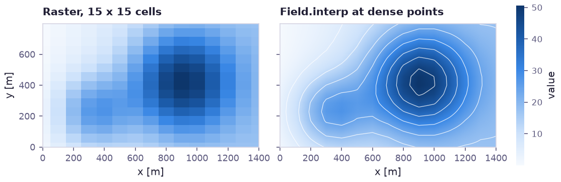
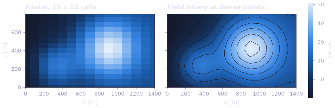
A 15 by 15 raster, for example exported from a solver, and the same field
read by Field.interp at dense query points.
- class prophys.structures.Field(values, frame, origin=(0.0, 0.0), cell=1.0, registry=None)[source]#
A scalar or vector raster on a regular 2D grid in frame, with bilinear interpolation.
values has shape
(ny, nx)for a scalar field or(ny, nx, c)for a vector field (such as windu, vcomponents withc=2). origin is the world coordinate(x, y)of the value at index(0, 0)and cell the grid spacing (scalar or(dx, dy)). Rows advance along the frame’s second axis (y) and columns along the first (x), matching the image array convention. The values may be an expression, such as a Param raster to calibrate.- Parameters:
values (Any) –
(ny, nx)or(ny, nx, c)grid values.frame (Frame) – Coordinate frame of the raster.
origin (tuple[float, float]) – World coordinate
(x, y)of the value at index(0, 0).cell (float | tuple[float, float]) – Grid spacing, a scalar or
(dx, dy).registry – Frame registry used to align query points.
Example:
terrain = prp.Field(elevation, site, origin=(0.0, 0.0), cell=25.0)
z = terrain.interp(houses)  # shape (n,)
- interp(points)[source]#
Bilinearly interpolate the field at points.
Queries outside the raster clamp to its edge cells. Differentiable in both the field values and the point coordinates.
- gradient()[source]#
Return the spatial gradient of a scalar field by finite differences, as a Field with 2 channels.
The channels are
(d/dy, d/dx)on the same grid, with central differences inside and one sided differences at the edges.- Return type:
Grid#
A fixed rectangular candidate domain — not itself part of the probabilistic model, but the standard way to evaluate an expression densely for a risk-map plot or a design search.
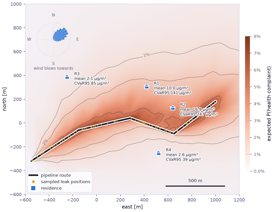
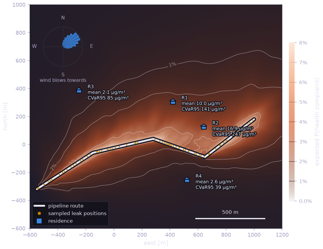
A risk map evaluated on a Grid in the pipeline-leak example
(:doc:`examples/gas_dispersion`).
- class prophys.structures.Grid(frame, x_range, y_range, nx, ny)[source]#
A regular 2D grid of candidate or evaluation points in frame.
Not itself an Expr (it is a fixed geometric domain, not part of the probabilistic model), but
positions()returns a PointList that can be fed into any structure or primitive.- Parameters:
Example:
grid = prp.Grid(site, (0.0, 1000.0), (0.0, 600.0), nx=16, ny=15)
d = grid.positions().closest_distance(turbines).evaluate()  # (ny * nx,)
d_map = d.reshape(grid.shape())                             # (ny, nx)
- positions()[source]#
Return all
ny * nxgrid points as a PointList, row by row with x varying fastest.- Return type:
- shape()[source]#
Return the grid shape
(ny, nx), for reshaping values evaluated atpositions().
Network#
A directed graph in a shared frame: nodes are a PointList
(coordinates may be a Param, so siting is optimizable), edges are a
fixed (m, 2) connectivity array, and each edge carries an optional
transmission weight — any expression, commonly a
BinaryState when whether a link is reinforced,
open, or online is itself a design decision. Network models supply
chains, power grids, and pipeline networks where risk cascades along
edges: edge_lengths() gives per-edge
distances (cable/pipe cost), as_lines()
exposes the edges as a LineList for
proximity queries (e.g. distance from a house to the nearest line), and
propagate() runs a differentiable
multi-hop cascade of a per-node signal (a fault, a contamination front, a
load spike) along the directed edges, decaying or amplifying at each hop
according to the edge weights.
- class prophys.structures.Network(nodes, edges, frame, weights=None, registry=None)[source]#
A directed graph embedded in frame, with optional transmission weights on its edges.
nodes is a PointList or raw
(n, ndim)coordinates, which may be a Param so node positions can be optimized. edges is a fixed(m, 2)integer array of (src, dst) node indices, since connectivity is structure, not a differentiable quantity. weights is an optional(m,)transmission factor per edge (any Expr, such as a Param or a vector of BinaryState instances stacked withprophys.stack()), 1 on every edge by default.Evaluating a Network yields its node coordinates, so it nests inside other expressions like a PointList does.
- Parameters:
nodes (Any) – A PointList (which supplies its own frame) or
(n, ndim)node coordinates.edges (Any) –
(m, 2)integer(src, dst)node indices.frame (Frame) – Coordinate frame (ignored when nodes is a PointList).
weights (Any) – Optional
(m,)transmission factors, one per edge.registry – Frame registry used to align query points.
- Raises:
ValueError – If edges is not
(m, 2).
Example:
w = prp.Param("w", shape=(3,), init=jnp.full(3, 0.8), bounds=(0.0, 1.0))
net = prp.Network(substations, edges=[[0, 1], [1, 2], [1, 3]], frame=site, weights=w)
load = net.propagate(source=jnp.array([1.0, 0.0, 0.0, 0.0]), steps=3)
- edge_lengths()[source]#
Return the Euclidean length of each edge, shape
(m,), differentiable in the node coordinates.- Return type:
- total_length()[source]#
Return the total edge length (such as cable or pipe cost), shape
().- Return type:
- as_lines()[source]#
Return the edges as a LineList of segments
(m, 2, ndim).Every segment primitive (closest_distance, distance_matrix, …) then works on the network geometry, such as the distance from houses to the nearest power line.
- Return type:
- propagate(source, steps=1, weights=None)[source]#
Cascade a signal on the nodes along the directed edges and return the accumulated signal.
Propagates source (shape
(n,)) for steps hops and returnssum_{k=0..steps} (M_w)^k source, shape(n,), whereM_w[dst, src] = w_efor each edgee. Thek=0term is the source itself. weights overrides the network’s own edge weights.Each hop multiplies by the transmission weight of the edge, so a failure, load or contamination signal decays (w < 1) or amplifies (w > 1) as it travels. Differentiable in both source and the weights. With BinaryState weights the cascade topology itself becomes a design variable.
Field3D / Grid3#
The volumetric counterparts of Field/Grid: a voxel raster on a
regular 3D grid with differentiable trilinear interpolation, and a dense
3D evaluation lattice. Used for subsurface property fields, 3D
concentration plumes, and atmospheric or thermal gradients where a single
2D slice isn’t enough.
- class prophys.structures.Field3D(values, frame, origin=(0.0, 0.0, 0.0), cell=1.0, registry=None)[source]#
A scalar or vector voxel raster on a regular 3D grid in frame, with trilinear interpolation.
values has shape
(nz, ny, nx)for a scalar field or(nz, ny, nx, c)for a vector field (such as a 3D flow withc=3). origin is the world coordinate(x, y, z)of voxel(0, 0, 0)and cell the voxel size (scalar or(dx, dy, dz)). The axis convention matches Field: the last array axis is x, then y, then z.- Parameters:
values (Any) –
(nz, ny, nx)or(nz, ny, nx, c)voxel values.frame (Frame) – Coordinate frame of the raster (
ndim=3).origin (tuple[float, float, float]) – World coordinate
(x, y, z)of voxel(0, 0, 0).cell (float | tuple[float, float, float]) – Voxel size, a scalar or
(dx, dy, dz).registry – Frame registry used to align query points.
- interp(points)[source]#
Trilinearly interpolate the field at points, a PointList of 3D coordinates.
Queries outside the raster clamp to its edge voxels.
- class prophys.structures.Grid3(frame, x_range, y_range, z_range, nx, ny, nz)[source]#
A regular 3D lattice of evaluation positions in frame.
The volumetric counterpart of Grid, for sampling a Field3D densely or defining a 3D lattice of design candidates. Not itself an Expr.
- Parameters:
frame (Frame) – Coordinate frame (
ndim=3).x_range (tuple[float, float]) –
(min, max)extent along x, endpoints included.y_range (tuple[float, float]) –
(min, max)extent along y, endpoints included.z_range (tuple[float, float]) –
(min, max)extent along z, endpoints included.nx (int) – Number of positions along x.
ny (int) – Number of positions along y.
nz (int) – Number of positions along z.
Mesh#
An unstructured triangular mesh carrying a per-vertex scalar field, with
differentiable barycentric (P1 finite-element) interpolation — the
ingestion point for FEM/CFD solver outputs (stress, pressure,
concentration) into a prophys graph. The mesh connectivity and vertex
positions are fixed structure; the field values (and query points) stay
differentiable, so a mesh-sampled physics surrogate can be calibrated
against observations exactly like any other attribute.
- class prophys.structures.Mesh(vertices, triangles, values, frame, registry=None)[source]#
A fixed 2D triangulation in frame carrying a scalar field at its vertices, with P1 interpolation.
vertices is a fixed
(v, 2)coordinate array and triangles a fixed(t, 3)integer connectivity array: the mesh is structure. values is the(v,)field at the vertices and may be any Expr (a Param makes the field itself calibratable against point observations). Interpolation is piecewise linear (the FEM P1 basis): exact at vertices, linear inside each triangle, and linearly extrapolated outside the mesh from the triangle the point is least outside of, so gradients stay defined everywhere.- Parameters:
vertices (Any) –
(v, 2)vertex coordinates.triangles (Any) –
(t, 3)vertex indices of each triangle.values (Any) –
(v,)field values at the vertices, an array or an expression.frame (Frame) – Coordinate frame of the mesh.
registry – Frame registry used to align query points.
- Raises:
ValueError – If vertices is not
(v, 2)or triangles is not(t, 3).
- interp(points)[source]#
Interpolate the vertex field at points barycentrically, shape
(n,).Differentiable in the field values and the query points (with a constant spatial gradient inside each triangle).