Distributions#
Every distribution below implements log_prob, a reparameterized
sample where possible, and closed-form mean/variance where they
exist. Parameters may themselves be
Expr (typically Param),
so a distribution’s shape can be learned or driven by upstream geometry.
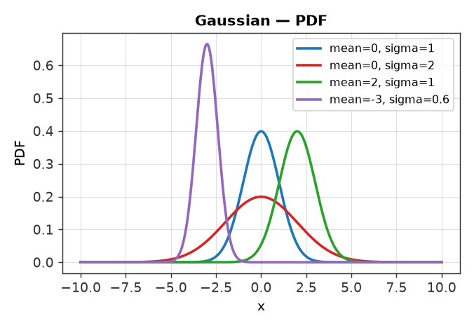
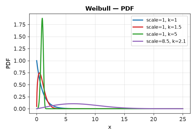
Each family below is shown with its probability-density plots and, where
useful, parameter-sensitivity sweeps.
The cumulative distribution cdf and its inverse quantile are mutual
duals: a distribution provides whichever it has in closed form and the
other is derived from it by a shared, differentiable monotone root-find (a
bracket-expanding bisection with implicit-function-theorem gradients). A
distribution therefore never needs both hand-written — supplying one is
enough for it to serve as a copula marginal (needs cdf) and as a
reparameterized sample source or process innovation (needs quantile).
Univariate#
Gaussian(mean, sigma)
Weibull(scale, concentration)
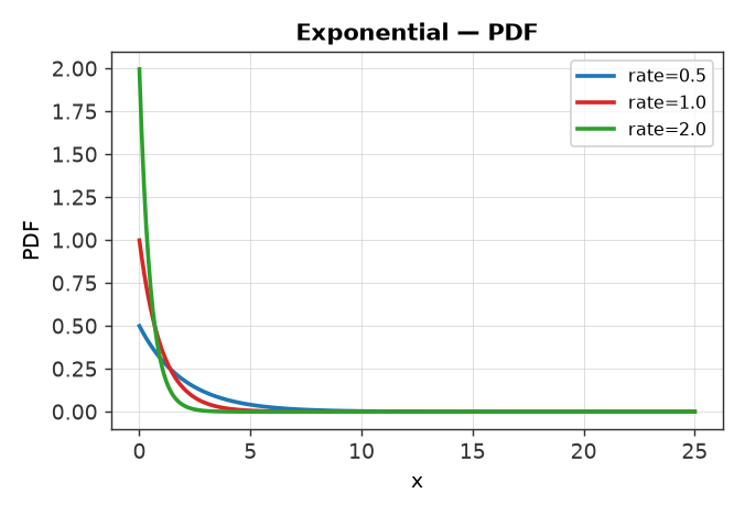
Exponential(rate)
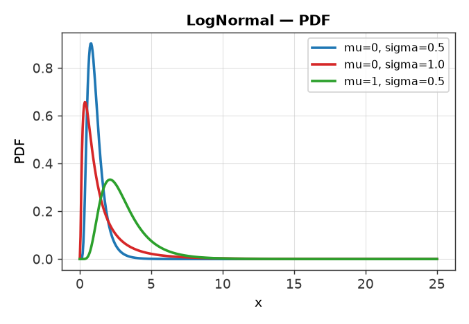
LogNormal(mu, sigma)
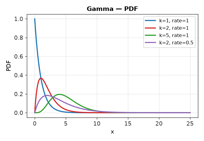
Gamma(concentration, rate)
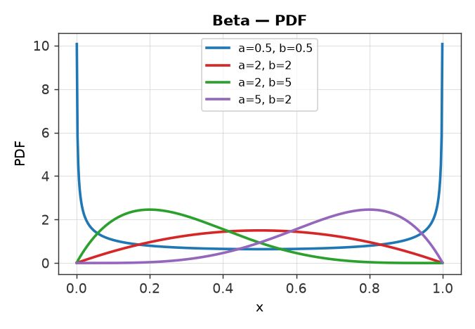
Beta(alpha, beta)
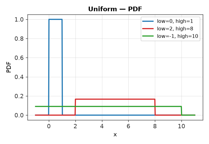
Uniform(low, high)
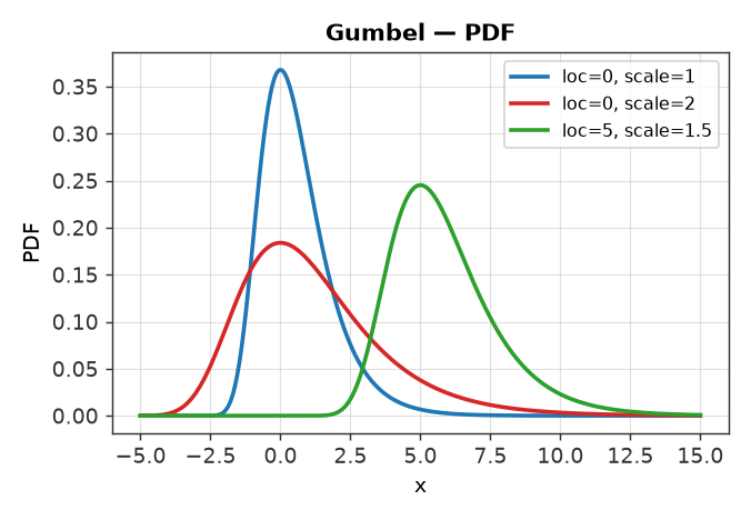
Gumbel(loc, scale)
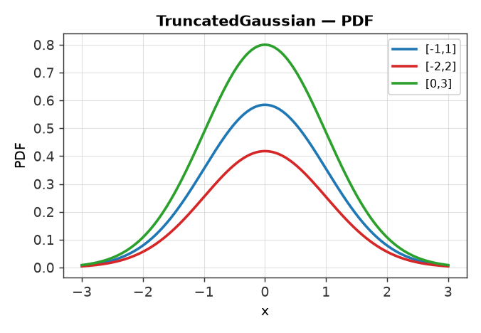
TruncatedGaussian(mean, sigma, low, high)
Parameter sensitivity#
Each univariate distribution also has a small-multiples sensitivity panel and per-parameter sweeps, e.g.:
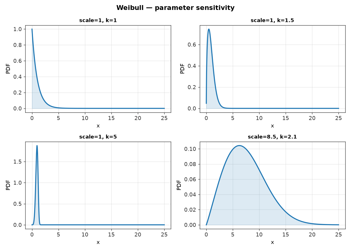
Weibull — parameter sensitivity grid
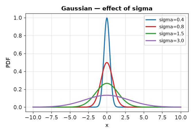
Gaussian — effect of sigma
Cumulative distributions#
Gaussian, Weibull, Exponential, LogNormal, Uniform, and Gumbel provide both
a closed-form cdf and a closed-form quantile; families that give
only one have the other filled in by inversion, and families that provide
neither (Gamma, Beta) raise on both. Gamma and Beta still
have reparameterized sample, so they work in Monte Carlo models and
calibration.
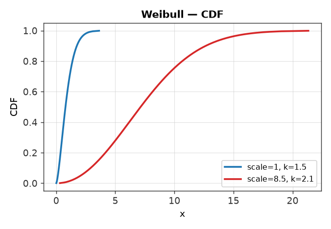
Weibull — CDF (closed-form quantile)
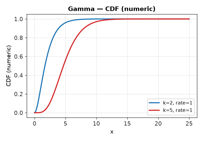
Gamma — CDF (numeric)
- class prophys.distributions.Gaussian(mean=0.0, sigma=1.0)[source]#
Normal distribution with mean mean and standard deviation sigma.
p(x) = exp(-(x - mean)^2 / (2 sigma^2)) / (sigma sqrt(2 pi)). Provides log_prob, cdf, quantile, reparameterized sample, mean and variance.- Parameters:
mean (Any) – Mean (location), any expression.
sigma (Any) – Standard deviation, positive.
Example:
noise = prp.Gaussian(0.0, prp.Param("sigma", init=0.5, transform="softplus"))
- log_prob(x)[source]#
Return the log density (or log mass for discrete families) at x, as an expression.
- sample(key, shape=())[source]#
Return random draws of shape shape (broadcast with the parameter shape), as an expression.
Families with a quantile sample by pushing uniforms through it, so draws are reparameterized and differentiable in the parameters. Gamma and Beta use implicit reparameterization instead, and discrete families are not differentiable in their parameters.
- class prophys.distributions.Weibull(scale=1.0, concentration=1.0)[source]#
Weibull distribution in scale and shape form:
p(x) = (k/lam) (x/lam)^(k-1) exp(-(x/lam)^k).The usual model for wind speeds and failure times. Provides log_prob, cdf, quantile, reparameterized sample and mean (
lam * Gamma(1 + 1/k)).- Parameters:
scale (Any) – Scale
lam, positive, in the units of x.concentration (Any) – Shape
k, positive.
Example:
wind = prp.Weibull(scale=8.5, concentration=2.1) # m/s
- log_prob(x)[source]#
Return the log density (or log mass for discrete families) at x, as an expression.
- sample(key, shape=())[source]#
Return random draws of shape shape (broadcast with the parameter shape), as an expression.
Families with a quantile sample by pushing uniforms through it, so draws are reparameterized and differentiable in the parameters. Gamma and Beta use implicit reparameterization instead, and discrete families are not differentiable in their parameters.
- class prophys.distributions.Exponential(rate=1.0)[source]#
Exponential distribution with rate rate:
p(x) = rate exp(-rate x)forx >= 0.Provides log_prob, cdf, quantile, reparameterized sample, mean (
1/rate) and variance (1/rate^2).- Parameters:
rate (Any) – Rate parameter, positive (inverse of the mean).
- log_prob(x)[source]#
Return the log density (or log mass for discrete families) at x, as an expression.
- sample(key, shape=())[source]#
Return random draws of shape shape (broadcast with the parameter shape), as an expression.
Families with a quantile sample by pushing uniforms through it, so draws are reparameterized and differentiable in the parameters. Gamma and Beta use implicit reparameterization instead, and discrete families are not differentiable in their parameters.
- quantile(q)[source]#
Return the quantile function (inverse CDF)
F^{-1}(q)forq in (0, 1), as an expression.Families without a closed form derive it by numerically inverting cdf from the bracket
[-1, 1], expanded as needed. A q the expanded bracket cannot reach gives NaN.
- class prophys.distributions.LogNormal(mu=0.0, sigma=1.0)[source]#
Log normal distribution:
log Xis Gaussian with mean mu and standard deviation sigma.Provides log_prob, cdf, quantile, reparameterized sample and mean (
exp(mu + sigma^2 / 2)).- Parameters:
mu (Any) – Mean of
log X.sigma (Any) – Standard deviation of
log X, positive.
- log_prob(x)[source]#
Return the log density (or log mass for discrete families) at x, as an expression.
- sample(key, shape=())[source]#
Return random draws of shape shape (broadcast with the parameter shape), as an expression.
Families with a quantile sample by pushing uniforms through it, so draws are reparameterized and differentiable in the parameters. Gamma and Beta use implicit reparameterization instead, and discrete families are not differentiable in their parameters.
- class prophys.distributions.Gamma(concentration=1.0, rate=1.0)[source]#
Gamma distribution with shape concentration and rate rate.
p(x) = rate^k x^(k-1) exp(-rate x) / Gamma(k)forx > 0. Provides log_prob, reparameterized sample, mean (k/rate) and variance (k/rate^2). Draws are differentiable in both parameters (implicit reparameterization of the gamma sampler).- Parameters:
concentration (Any) – Shape
k, positive.rate (Any) – Rate, positive (inverse scale).
- log_prob(x)[source]#
Return the log density (or log mass for discrete families) at x, as an expression.
- sample(key, shape=())[source]#
Return random draws of shape shape (broadcast with the parameter shape), as an expression.
Families with a quantile sample by pushing uniforms through it, so draws are reparameterized and differentiable in the parameters. Gamma and Beta use implicit reparameterization instead, and discrete families are not differentiable in their parameters.
- class prophys.distributions.Beta(alpha=1.0, beta=1.0)[source]#
Beta distribution on
(0, 1)with shape parameters alpha and beta.Provides log_prob, reparameterized sample, mean (
alpha / (alpha + beta)) and variance. Draws are differentiable in both parameters (implicit reparameterization, computed in log space so small shape parameters do not underflow).- Parameters:
alpha (Any) – First shape parameter, positive.
beta (Any) – Second shape parameter, positive.
- log_prob(x)[source]#
Return the log density (or log mass for discrete families) at x, as an expression.
- sample(key, shape=())[source]#
Return random draws of shape shape (broadcast with the parameter shape), as an expression.
Families with a quantile sample by pushing uniforms through it, so draws are reparameterized and differentiable in the parameters. Gamma and Beta use implicit reparameterization instead, and discrete families are not differentiable in their parameters.
- class prophys.distributions.Uniform(low=0.0, high=1.0)[source]#
Continuous uniform distribution on
[low, high].Provides log_prob, cdf, quantile, reparameterized sample and mean.
- Parameters:
low (Any) – Lower bound.
high (Any) – Upper bound, greater than low.
- log_prob(x)[source]#
Return the log density (or log mass for discrete families) at x, as an expression.
- sample(key, shape=())[source]#
Return random draws of shape shape (broadcast with the parameter shape), as an expression.
Families with a quantile sample by pushing uniforms through it, so draws are reparameterized and differentiable in the parameters. Gamma and Beta use implicit reparameterization instead, and discrete families are not differentiable in their parameters.
- class prophys.distributions.Gumbel(loc=0.0, scale=1.0)[source]#
Gumbel (type I extreme value) distribution for maxima, with location loc and scale scale.
F(x) = exp(-exp(-(x - loc) / scale)). The usual model for annual maxima of floods, winds and loads. Provides log_prob, cdf, quantile and reparameterized sample.- Parameters:
loc (Any) – Location (mode).
scale (Any) – Scale, positive.
- log_prob(x)[source]#
Return the log density (or log mass for discrete families) at x, as an expression.
- sample(key, shape=())[source]#
Return random draws of shape shape (broadcast with the parameter shape), as an expression.
Families with a quantile sample by pushing uniforms through it, so draws are reparameterized and differentiable in the parameters. Gamma and Beta use implicit reparameterization instead, and discrete families are not differentiable in their parameters.
- class prophys.distributions.TruncatedGaussian(mean=0.0, sigma=1.0, low=-inf, high=inf)[source]#
Gaussian with a log density renormalized to the interval
[low, high].Only log_prob is truncated: it is the Gaussian log density minus
log(Phi((high - mean)/sigma) - Phi((low - mean)/sigma)), and it does not return-infoutside the interval, so use it as a likelihood for data known to lie in[low, high]. sample, cdf, quantile, mean and variance are those of the untruncated parentGaussian.- Parameters:
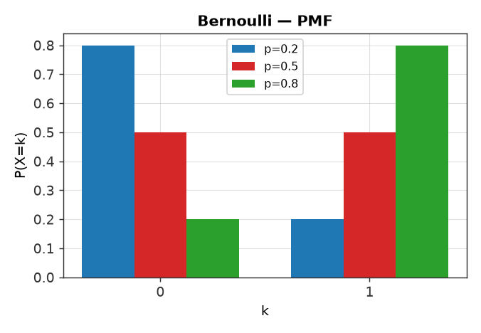
- class prophys.distributions.Bernoulli(prob=0.5)[source]#
Bernoulli distribution over
{0, 1}with success probability prob.Provides log_prob, mean and sample. Draws are 0.0 or 1.0 floats and are not differentiable in prob.
- Parameters:
prob (Any) – Probability of 1, in
[0, 1].
- log_prob(x)[source]#
Return the log density (or log mass for discrete families) at x, as an expression.
- sample(key, shape=())[source]#
Return random draws of shape shape (broadcast with the parameter shape), as an expression.
Families with a quantile sample by pushing uniforms through it, so draws are reparameterized and differentiable in the parameters. Gamma and Beta use implicit reparameterization instead, and discrete families are not differentiable in their parameters.
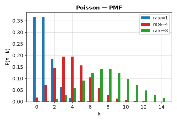
- class prophys.distributions.Poisson(rate=1.0)[source]#
Poisson distribution over nonnegative integer counts with mean rate.
Provides log_prob, mean and sample. Draws are counts stored as floats and are not differentiable in rate.
- Parameters:
rate (Any) – Expected count, positive.
- log_prob(x)[source]#
Return the log density (or log mass for discrete families) at x, as an expression.
- sample(key, shape=())[source]#
Return random draws of shape shape (broadcast with the parameter shape), as an expression.
Families with a quantile sample by pushing uniforms through it, so draws are reparameterized and differentiable in the parameters. Gamma and Beta use implicit reparameterization instead, and discrete families are not differentiable in their parameters.
- class prophys.distributions.Categorical(probs)[source]#
Categorical distribution over k categories, indexed from 0, with probabilities probs.
Provides sample (integer indices) and log_prob (at integer indices).
- Parameters:
probs (Any) –
(..., k)probabilities along the last axis, summing to 1.
- sample(key, shape=())[source]#
Return random draws of shape shape (broadcast with the parameter shape), as an expression.
Families with a quantile sample by pushing uniforms through it, so draws are reparameterized and differentiable in the parameters. Gamma and Beta use implicit reparameterization instead, and discrete families are not differentiable in their parameters.
Circular#
For angular quantities like wind direction, where ordinary Gaussians are wrong because \(0\) and \(2\pi\) are the same point.
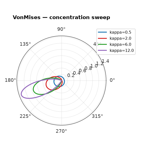
Higher kappa -> more concentrated around loc.
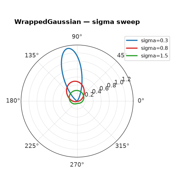
A Gaussian wrapped onto the circle.
- class prophys.distributions.VonMises(loc=0.0, kappa=1.0)[source]#
Von Mises distribution on the circle (radians), the circular analog of a Gaussian.
locis the mean direction,kappathe concentration (kappanear 0 is uniform, largekappaconcentrates at loc). Provides log_prob, sample (by rejection sampling, NaN in the rare event that no round accepts) and mean (the mean direction).- Parameters:
loc (Any) – Mean direction in radians.
kappa (Any) – Concentration, nonnegative.
Example:
direction = prp.VonMises(loc=prp.deg2rad(240.0), kappa=2.5)
- log_prob(x)[source]#
Return the log density (or log mass for discrete families) at x, as an expression.
- sample(key, shape=())[source]#
Return random draws of shape shape (broadcast with the parameter shape), as an expression.
Families with a quantile sample by pushing uniforms through it, so draws are reparameterized and differentiable in the parameters. Gamma and Beta use implicit reparameterization instead, and discrete families are not differentiable in their parameters.
- class prophys.distributions.WrappedGaussian(loc=0.0, sigma=1.0, n_wraps=3)[source]#
Gaussian wrapped onto the circle, for angular quantities in radians.
The log density sums n_wraps wrapped copies on each side of loc, which is accurate for sigma well below
2*pi. Provides log_prob.- Parameters:
loc (Any) – Mean direction in radians.
sigma (Any) – Standard deviation of the unwrapped Gaussian, in radians.
n_wraps (int) – Number of wraps summed on each side.
Directional climatologies#
DirectionalMixture is the standard
representation of a directional climatology — wind rose, wave rose,
current regime, or any other joint distribution of “which direction” and
“how strong”: the circle is divided into sectors, each with an occurrence
weight, a circular spread (a VonMises
around the sector center), and its own conditional intensity distribution
(e.g. a per-sector Weibull of wind
speed). All parameters — sector weights, spreads, and every conditional
intensity distribution’s parameters — are ordinary Exprs, so a
climatology can be built from met-mast or reanalysis observations with
directional_mixture() (see Reading Data), refined against
the same data inside a model, and its sector weights can just as well
be design variables (e.g. trading off wake losses against a
site’s directional wind resource).
import jax.numpy as jnp
import prophys as prp

sector_speeds = [
    prp.Weibull(scale=prp.Param(f"scale_{i}", init=7.0), concentration=2.0)
    for i in range(8)
]
wind_rose = prp.DirectionalMixture.evenly_spaced(
    weights=prp.Param("sector_weights", shape=(8,), init=jnp.full((8,), 1 / 8)),
    intensities=sector_speeds,
)
wind_rose.log_prob(direction=jnp.deg2rad(200.0), intensity=9.5)
- class prophys.distributions.DirectionalMixture(directions, concentrations, intensities, logits)[source]#
Joint distribution of a direction and a conditional intensity, such as a wind rose.
The standard representation of directional climatologies (wind or wave climate, current regimes, directional seismic loading): the circle is divided into k directional sectors, each with an occurrence weight, a von Mises spread around its center direction, and its own conditional intensity distribution (such as a Weibull of wind speed per sector). All parameters may be expressions, so the whole climatology can be calibrated against observed
(angle, intensity)pairs with fit_distribution.- Parameters:
directions (Any) – Sector center angles in radians, shape
(k,).concentrations (Any) – Von Mises concentration per sector, shape
(k,)(higher is narrower, may be a learnable Param).intensities (Sequence[Distribution]) – k conditional intensity distributions, one per sector.
logits (Any) – Unnormalized sector occurrence log weights, shape
(k,)(normalized internally by softmax, may be a learnable Param).
Example:
rose = prp.DirectionalMixture.evenly_spaced(
    weights=sector_freq,  # (12,) observed sector frequencies
    intensities=[prp.Weibull(scale=s, concentration=2.0) for s in sector_scale],
)
- classmethod evenly_spaced(weights, intensities, concentration=None)[source]#
Build a climatology with k sectors evenly spaced around the circle.
Sector 0 is centered at angle 0 and k is the number of intensities, at least 2.
- Parameters:
weights (Any) – Sector occurrence weights, shape
(k,), such as observed sector frequencies (normalized internally).intensities (Sequence[Distribution]) – k conditional intensity distributions.
concentration (Any) – Von Mises concentration per sector. Defaults to
1 / sigma**2withsigmahalf a sector width, a spread that roughly tiles the circle.
- Raises:
ValueError – If fewer than 2 intensities are given.
- Return type:
- log_prob(direction, intensity)[source]#
Return the joint log density of
(direction, intensity)pairs, elementwise over the inputs.
- sample(key, shape=())[source]#
Draw
(direction, intensity)pairs, shapeshape + (2,).Each draw picks a sector by its occurrence weight, then samples the sector’s direction spread and its conditional intensity.
Multivariate & mixtures#
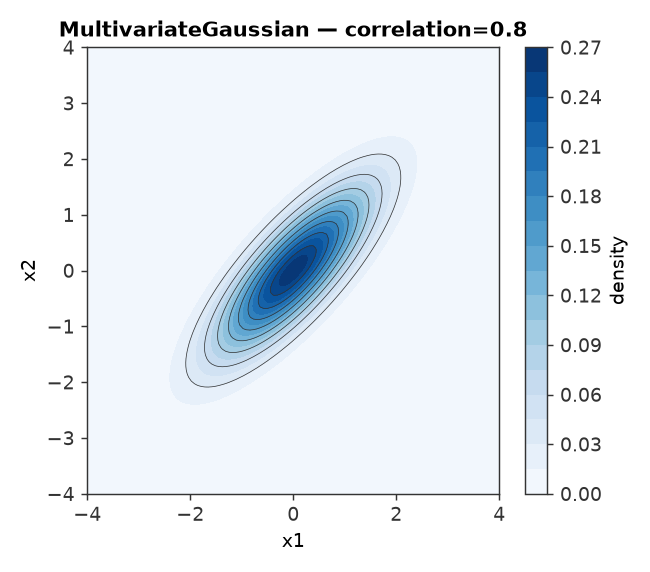
Cholesky-parameterized covariance — always positive-definite under gradient updates.
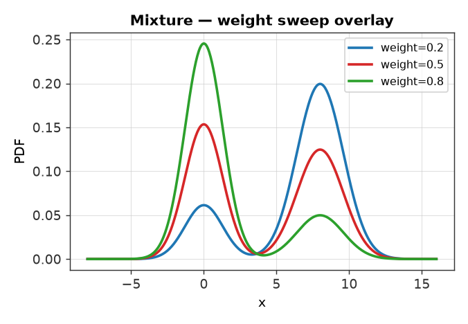
Finite mixture with softmax-normalized weights. Its cdf is the
weight-averaged component CDFs (strictly increasing), so the derived
quantile is unambiguous — a mixture can serve as a copula
marginal or as an autoregressive process’s innovation.
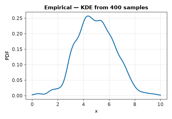
Kernel-density estimate from raw samples — stays differentiable.
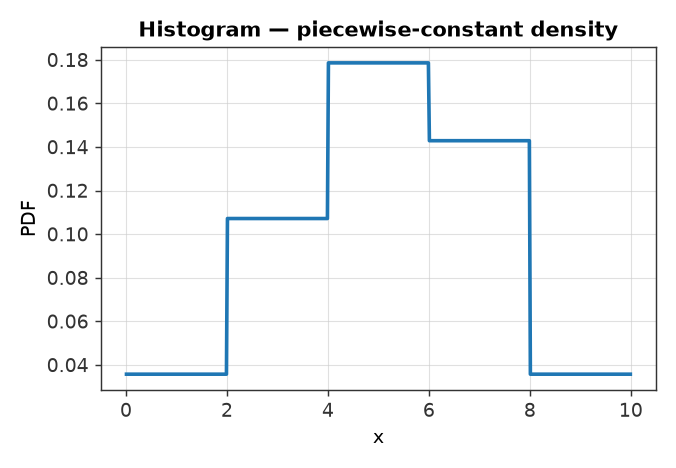
Piecewise-constant density from bin edges/probabilities.
- class prophys.distributions.MultivariateGaussian(mean, cholesky)[source]#
Multivariate normal distribution parameterized by its mean and the Cholesky factor of its covariance.
Values have the dimension axis last. Provides log_prob, reparameterized sample (shape
(*shape, d)) and mean.- Parameters:
mean (Any) – Mean vector, shape
(d,).cholesky (Any) – Lower triangular factor
Lof the covariance (cov = L @ L.T), shape(d, d). Parameterizing via the Cholesky factor keeps the covariance positive definite under gradient updates.
- log_prob(x)[source]#
Return the log density (or log mass for discrete families) at x, as an expression.
- sample(key, shape=())[source]#
Return random draws of shape shape (broadcast with the parameter shape), as an expression.
Families with a quantile sample by pushing uniforms through it, so draws are reparameterized and differentiable in the parameters. Gamma and Beta use implicit reparameterization instead, and discrete families are not differentiable in their parameters.
- class prophys.distributions.Mixture(components, logits)[source]#
Finite mixture of component distributions with (possibly learnable) weights.
The weights are
softmax(logits). Provides log_prob, cdf (and hence quantile), sample and mean wherever the components do.- Parameters:
components (Sequence[Distribution]) – Component distributions.
logits (Any) – Unnormalized log weights, shape
(k,), may be a Param.
Example:
bimodal = prp.Mixture([prp.Gaussian(2.0, 0.5), prp.Gaussian(6.0, 1.0)], logits=jnp.log(jnp.array([0.7, 0.3])))
- log_prob(x)[source]#
Return the log density (or log mass for discrete families) at x, as an expression.
- class prophys.distributions.Empirical(samples, bandwidth=0.1)[source]#
Data driven distribution defined by a fixed sample set, such as observed wind speeds.
log_prob uses kernel density estimation (Gaussian kernel with the given bandwidth), so it stays differentiable. sample resamples the data with replacement, and mean is the sample mean.
- Parameters:
samples (Any) – Observed values, shape
(n,).bandwidth (float) – Kernel standard deviation, in the units of the data.
- log_prob(x)[source]#
Return the log density (or log mass for discrete families) at x, as an expression.
- sample(key, shape=())[source]#
Return random draws of shape shape (broadcast with the parameter shape), as an expression.
Families with a quantile sample by pushing uniforms through it, so draws are reparameterized and differentiable in the parameters. Gamma and Beta use implicit reparameterization instead, and discrete families are not differentiable in their parameters.
- class prophys.distributions.Histogram(edges, probs)[source]#
Piecewise constant density over histogram bins.
Provides log_prob, differentiable in probs. The bin probabilities are normalized internally, and values outside the edges take the density of the nearest end bin.
- Parameters:
edges (Any) – Increasing bin edges, shape
(n + 1,).probs (Any) – Bin probabilities or counts, shape
(n,).
Copulas & dependence structures#
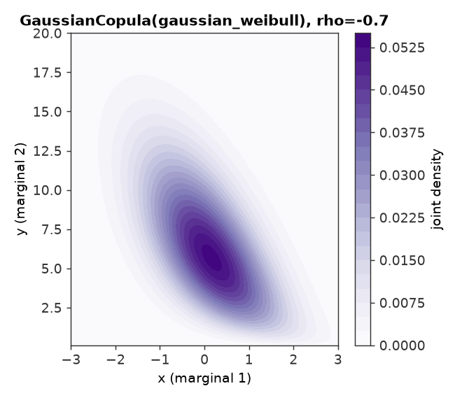
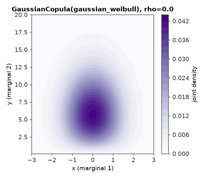
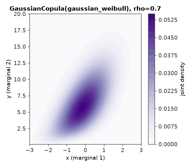
A GaussianCopula couples arbitrary
marginals (each needs a cdf for the density and a quantile for
sampling — either closed-form or derived, so a
Mixture marginal works too) through a
correlation matrix that is parameterized so it is always valid — an
unconstrained gradient step can never produce a non-positive-definite
correlation matrix.
- class prophys.distributions.GaussianCopula(marginals, corr_raw)[source]#
Joint distribution coupling arbitrary marginals through a Gaussian copula.
Each marginal keeps its own distribution. The dependence is that of a multivariate normal with a correlation matrix parameterized by an unconstrained vector (see
corr_cholesky_from_raw()), so the vector may be a Param and remains a valid correlation matrix under any gradient step. Marginals must provide cdf (for log_prob) and quantile (for sample). log_prob takes a sequence of d values, one per marginal, and sample returns shape(*shape, d).- Parameters:
marginals (Sequence[Distribution]) – The d marginal distributions.
corr_raw (Any) – Unconstrained correlation vector of length
d * (d - 1) / 2.
Example:
joint = prp.GaussianCopula(
    [prp.Weibull(scale=8.0, concentration=2.0), prp.Gaussian(12.0, 4.0)],
    corr_raw=prp.Param("corr_raw", shape=(1,), init=jnp.zeros(1)),
)
met = prp.JointRandomVariable("met", joint, components=["speed", "temperature"])
- log_prob(x)[source]#
Return the log density (or log mass for discrete families) at x, as an expression.
- sample(key, shape=())[source]#
Draw joint samples of shape
(*shape, d), one column per marginal.Reparameterized: standard normals are correlated through the same Cholesky factor the log_prob kernel builds from corr_raw, mapped to uniforms by the normal CDF, then passed through each marginal’s quantile. Gradients flow to both corr_raw and every marginal parameter.
- class prophys.distributions.Correlation(marginal_a, marginal_b, rho_raw)[source]#
Bivariate Gaussian copula between two marginals, with correlation
rho = tanh(rho_raw).A convenience over
GaussianCopulafor two variables. log_prob takes a pair(a, b)and sample returns shape(*shape, 2).- Parameters:
marginal_a (Distribution) – Distribution of the first variable.
marginal_b (Distribution) – Distribution of the second variable.
rho_raw (Any) – Unconstrained scalar. The copula correlation is
tanh(rho_raw).
- log_prob(x)[source]#
Return the log density (or log mass for discrete families) at x, as an expression.
- sample(key, shape=())[source]#
Return random draws of shape shape (broadcast with the parameter shape), as an expression.
Families with a quantile sample by pushing uniforms through it, so draws are reparameterized and differentiable in the parameters. Gamma and Beta use implicit reparameterization instead, and discrete families are not differentiable in their parameters.
- class prophys.distributions.Independent(marginals)[source]#
Joint distribution of independent marginals (a product density).
Equivalent to a copula with zero correlation, provided for readability at call sites. log_prob takes a sequence of values, one per marginal, and sums their log densities. sample returns shape
(*shape, d).- Parameters:
marginals (Sequence[Distribution]) – The marginal distributions.
- log_prob(x)[source]#
Return the log density (or log mass for discrete families) at x, as an expression.
- sample(key, shape=())[source]#
Return random draws of shape shape (broadcast with the parameter shape), as an expression.
Families with a quantile sample by pushing uniforms through it, so draws are reparameterized and differentiable in the parameters. Gamma and Beta use implicit reparameterization instead, and discrete families are not differentiable in their parameters.
Discrete distributions#