

Example: Pipeline-Leak Community Health Risk#
This chapter builds a complete prophys model step by step. Its defining
idea: the hazard source is not a fixed point. A pipeline can fail
anywhere along its route, so the leak location is a continuous,
reparameterized random variable — not a hand-picked point. On top of that,
wind speed and direction are two more random inputs. All three are
marginalized out together by Monte Carlo, through a Gaussian-plume
dispersion model and a dose-response curve, to give the expected
health-complaint risk everywhere on the map and the tail exposure at
individual residences. The full runnable source is
examples/gas_dispersion/model.py.
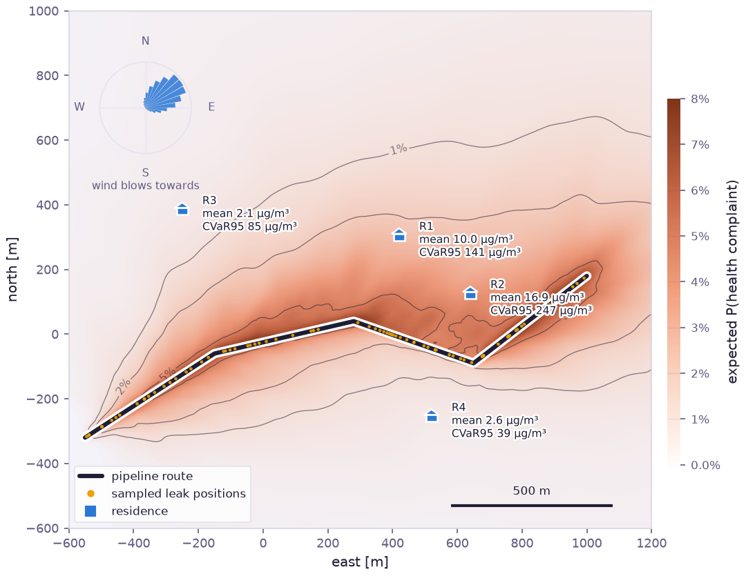
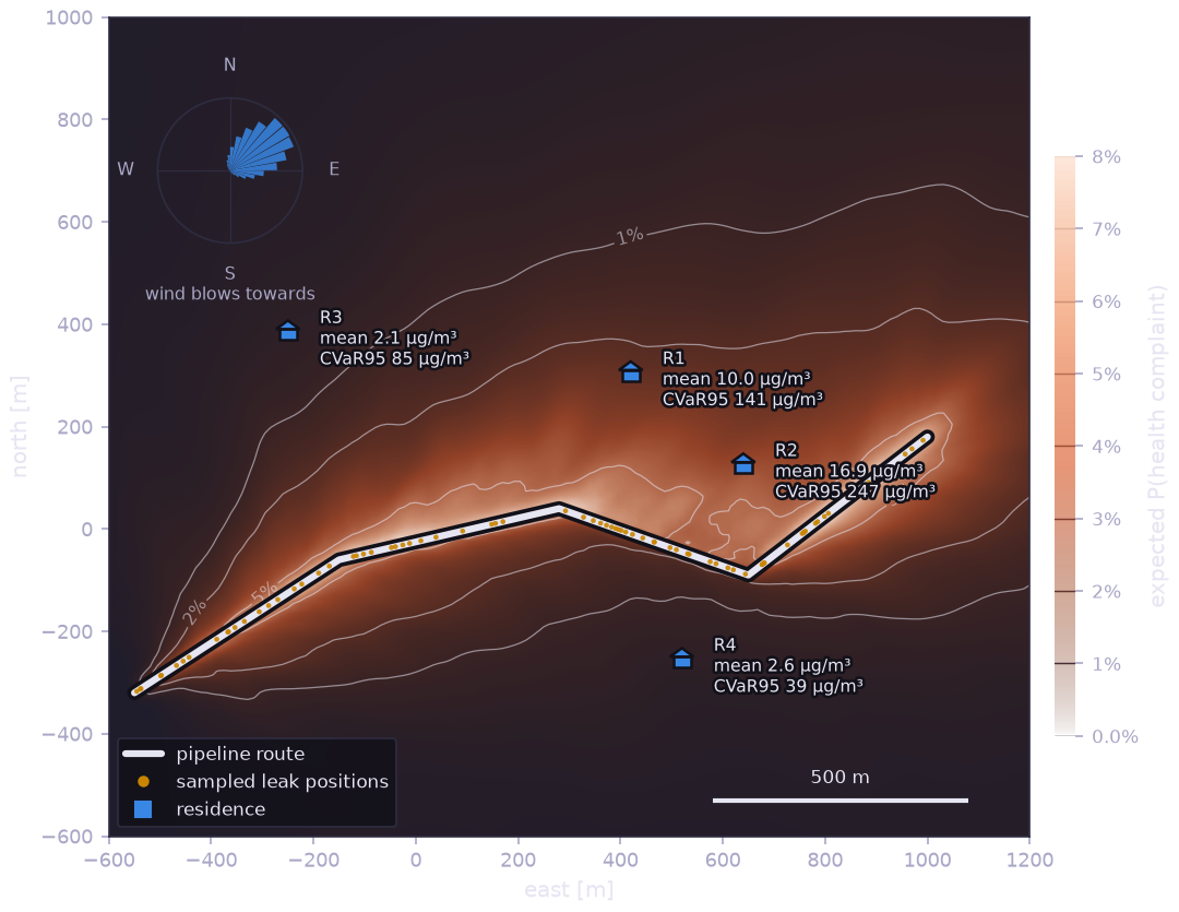
The marginalized risk landscape: the probability of a health complaint at every point of the site, averaged over 4 000 joint draws of the leak position along the route (dots, a subsample), the wind speed and the wind direction (rose, upper left). The hazard is smeared along the whole route and blown to the north-east, the direction the wind most often blows towards, with contours at 1, 2 and 5 %. Each residence is labelled with its mean exposure and the mean of its worst 5 % of draws (CVaR95): R2, closest downwind of the eastern segment, carries the highest tail exposure, R4 south of the route the lowest.
Step 1 — The route and receptors#
Everything spatial lives in one site frame. The pipeline is a
Polyline — a single connected route whose
vertices could themselves be a Param (optimizable
siting) — and the residences are a PointList:
site = prp.Frame("site", units="m")

pipeline = prp.Polyline(
    jnp.array(
        [
            [-550.0, -320.0],
            [-150.0, -60.0],
            [280.0, 40.0],
            [650.0, -90.0],
            [1000.0, 180.0],
        ]
    ),
    site,
)

residence_names = ["R1", "R2", "R3", "R4"]
residences = prp.PointList(
    jnp.array([[420.0, 300.0], [640.0, 120.0], [-250.0, 380.0], [520.0, -260.0]]), site
)
Step 2 — Uncertainty enters at the inputs#
The leak location is leak_frac ~ Uniform(0, 1) pushed through
Polyline.point_at — a
reparameterized draw of a position anywhere along the route, differentiable
in both the fractional arc-length and the route geometry. Wind speed is
Weibull, wind direction von Mises (the circular analog of a Gaussian — a
plain Gaussian would be wrong because 0° and 360° are the same direction):
leak_frac = prp.RandomVariable("leak_frac", prp.Uniform(0.0, 1.0))
wind_speed = prp.RandomVariable("wind_speed", prp.Weibull(scale=6.0, concentration=2.0))
wind_direction = prp.RandomVariable("wind_direction", prp.VonMises(loc=prp.deg2rad(35.0), kappa=3.0))

# Leak position anywhere along the route — reparameterized, differentiable
# in both the fractional arc-length draw and the route geometry.
leak_xy = pipeline.point_at(leak_frac)  # (2,) per sample
Every quantity downstream of these three leaves is itself random. The compiled model marginalizes them out by Monte Carlo, and — because all three sample by reparameterization — gradients flow through the marginalization back to any trainable parameter.
Step 3 — The physics: a Gaussian plume, symbolically#
Ground-level concentration follows the standard Gaussian dispersion model.
Each receptor is rotated into plume-aligned coordinates using the random
wind direction, the plume spread grows with downwind distance via
differentiable TableLookup1D
Pasquill–Gifford coefficients (stability class D), and the emission rate
carries a trainable, bounded abatement fraction:
sigma_y_table = prp.TableLookup1D(grid=[50.0, 200.0, 500.0, 1000.0, 2000.0], values=[8.0, 25.0, 55.0, 100.0, 180.0])
sigma_z_table = prp.TableLookup1D(grid=[50.0, 200.0, 500.0, 1000.0, 2000.0], values=[5.0, 15.0, 30.0, 50.0, 80.0])

release_height = 1.0  # ground-level pipeline release [m]
abatement = prp.Param("abatement", init=0.2, bounds=(0.0, 0.9))  # fraction of emissions removed
emission_rate = (1.0 - abatement) * prp.Param("emission_rate", init=5.0)  # g/s, optimizable via abatement


def plume_concentration(receptor_coords, source_xy) -> prp.Expr:
    delta = receptor_coords - source_xy
    dx, dy = delta[..., 0], delta[..., 1]

    theta = wind_direction  # radians the wind blows towards
    downwind = dx * prp.cos(theta) + dy * prp.sin(theta)
    crosswind = -dx * prp.sin(theta) + dy * prp.cos(theta)

    downwind_pos = prp.relu(downwind) + 1e-3
    sigma_y = sigma_y_table(downwind_pos)
    sigma_z = sigma_z_table(downwind_pos)

    u = prp.clip(wind_speed, 0.5, None)
    crosswind_term = prp.exp(-0.5 * (crosswind / sigma_y) ** 2)
    vertical_term = prp.exp(-0.5 * (release_height / sigma_z) ** 2)
    conc = (emission_rate / (2 * jnp.pi * u * sigma_y * sigma_z)) * crosswind_term * vertical_term
    return prp.where(downwind > 0, conc, 0.0)  # upwind receptors see no plume
Every line is symbolic — jax.grad differentiates through the rotation,
the table lookups, and the exponentials in one pass, and the whole thing is
shape-agnostic: the same function serves a single residence (broadcasting
against the Monte-Carlo sample axis) or a dense grid slice. A
PiecewiseLinear dose-response curve turns
the concentration into the probability of a health complaint.
Step 4 — Uncertain attributes, tail risk, and a correlation#
Exposure at a residence is LogNormal around the physical concentration (multiplicative monitoring noise with a learnable sigma). Because every attribute is marginalized over the joint (leak, wind) draws, the engine gives not just the expectation but the Conditional Value-at-Risk — the mean of the worst 5 % of outcomes:
conc_res = [plume_concentration(residences.coords[i], leak_xy) for i in range(len(residence_names))]

monitoring_noise_sigma = prp.Param("noise_sigma", init=0.3, transform="softplus")
exposures = [
    prp.UncertainAttribute(
        f"exposure_{name}",
        prp.LogNormal(mu=prp.log(prp.clip(conc_res[i], 1e-6, None)), sigma=monitoring_noise_sigma),
        unit="g/m3",
        domain=f"ground-level pollutant concentration at {name}",
    )
    for i, name in enumerate(residence_names)
]
and in run():
e = float(compiled.expectation(f"exposure_{name}"))
c95 = float(compiled.cvar(f"exposure_{name}", alpha=0.95))
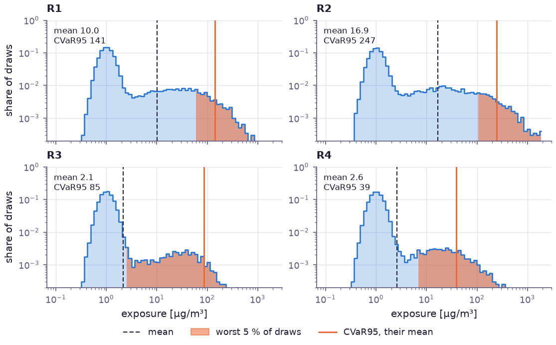
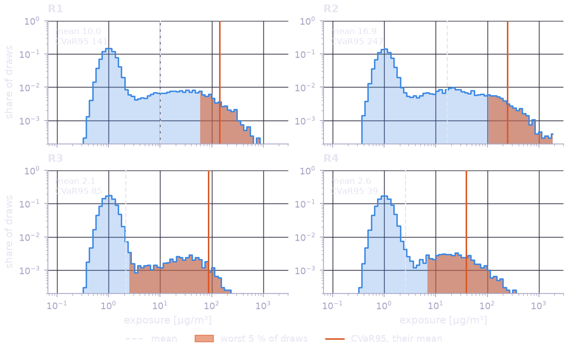
Exposure at each residence over 20 000 joint draws of leak and wind, on logarithmic axes. The narrow peak at 1 µg/m³ holds the draws in which the plume misses the residence: the model floors the concentration at 1e-6 g/m³ before the monitoring noise. The long right shoulder holds the draws in which it does not. The mean (dashed) says little about that shoulder; the CVaR95 (solid), the mean of the worst 5 % of draws (shaded), is ten to forty times larger.
Two nearby residences share the same weather and leak, so their exposures
are correlated even conditional on the mean model — captured with a
trainable Correlation (a bivariate Gaussian
copula) in an AttributeInteractions.
Step 5 — Risk landscape, calibration, design, export#
Because every quantity is an ordinary symbolic expression, evaluating it
over a dense Grid while sampling the same
random inputs turns it into the marginalized risk landscape at the top of
this page. risk_landscape draws the three random inputs, evaluates the
plume at all 25 600 grid cells for every draw and averages the
dose-response.
The compiled model then calibrates the monitoring-noise sigma against observed exposures at R1:
cal = prp.calibrate(
    compiled, "exposure_R1", synthetic_exposure,
    trainable=["noise_sigma"], n_steps=150, learning_rate=0.05,
)
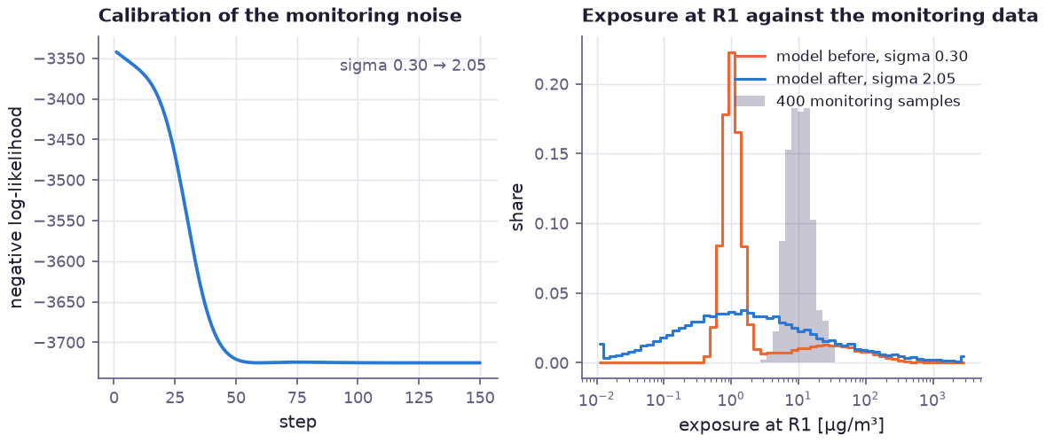
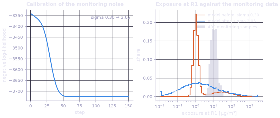
Left: the negative log-likelihood of the 400 monitoring samples while the noise sigma is fitted. Right: the exposure at R1 before and after, against the samples. Only the noise level is trainable, so the fit can widen the distribution but not move it: sigma grows from 0.30 to 2.05 to reach samples around 10 µg/m³, ten times the model’s typical value. A misfit this visible says that the emission rate, not only the noise, should be among the calibrated parameters.
Finally the abatement fraction is optimized to minimize the total
exposure at the four residences under a design scenario (a mid-route leak,
6 m/s wind blowing towards 30°). Its [0, 0.9] box is enforced
structurally by the bounded Param, not by a penalty:
total_exposure = (conc_res[0] + conc_res[1] + conc_res[2] + conc_res[3])[0]
result = prp.optimize(
    total_exposure,
    wrt=[p for p in model.params().values() if p.name == "abatement"],
    n_steps=120,
    learning_rate=0.5,
    extra_env={"leak_frac": 0.5, "wind_speed": 6.0, "wind_direction": jnp.deg2rad(30.0)},
)
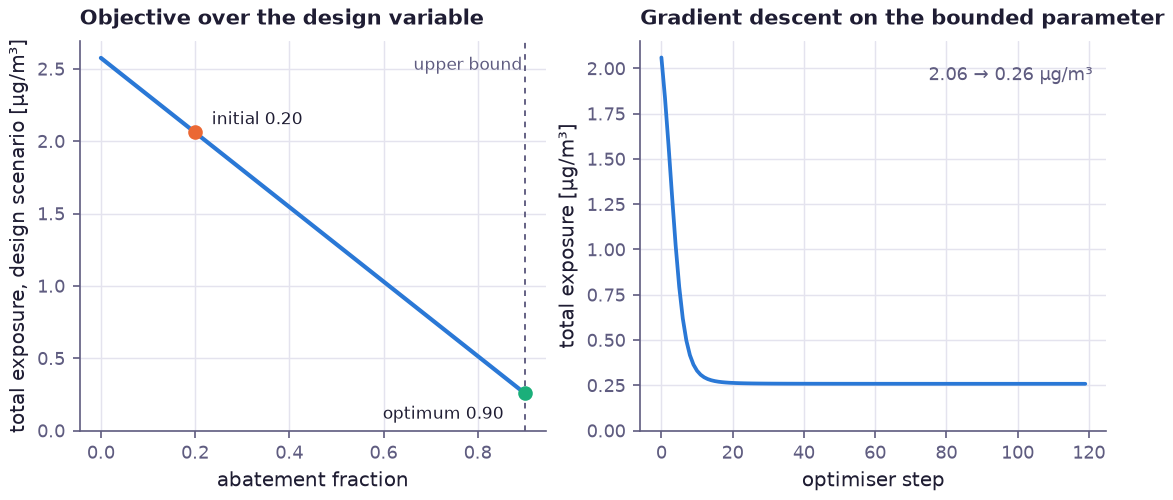
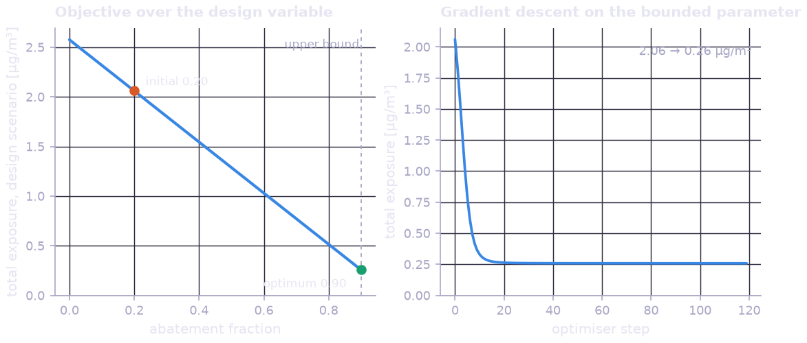
Left: the total exposure of the design scenario over the abatement fraction, linear in it because the emission rate is. With no cost on abatement the optimum is the upper bound. Right: the optimizer works on the unconstrained value behind the bounded parameter and approaches 0.9 without ever leaving the box, cutting the exposure from 2.06 to 0.26 µg/m³.
The model is exported to the neutral
ModelPackage.
Results#
The console output of python examples/gas_dispersion/model.py:
=== Expected and tail risk at residences (marginalized) ===
  R1: E[exposure]=1.00e-05 g/m3   CVaR95[exposure]=1.41e-04 g/m3
  R2: E[exposure]=1.69e-05 g/m3   CVaR95[exposure]=2.47e-04 g/m3
  R3: E[exposure]=2.14e-06 g/m3   CVaR95[exposure]=8.51e-05 g/m3
  R4: E[exposure]=2.56e-06 g/m3   CVaR95[exposure]=3.88e-05 g/m3
  P(complaint at R1) = 0.021978002041578293

=== Calibration ===
final loss: -3725.312744140625
fitted params: {'abatement': 0.20000000298023224, 'emission_rate': 5.0, 'noise_sigma': 2.0512874126434326}

=== Design optimization ===
initial total exposure: 2.060153519778396e-06
final total exposure: 2.582790159522119e-07
optimized abatement fraction: 0.8997059

=== Export ===
exported attributes: ['exposure_R1', 'exposure_R2', 'exposure_R3', 'exposure_R4', 'complaint_R1']
pipeline length [m]: 1752.763427734375
Primitives exercised#
Category |
Used for |
|---|---|
The pipeline route; |
|
Residence receptors; dense risk-map evaluation |
|
Leak location, wind speed, and wind direction as |
|
Dispersion coefficients; dose-response |
|
Exposure noise; complaint likelihood; shared-weather coupling |
|
|
Expected & tail risk, training, design, export |
Running it#
$ python examples/gas_dispersion/model.py