Example: Distribution-Grid Reinforcement

This chapter builds a small electricity distribution network — one substation feeding several load nodes over a directed graph — where a fault at the substation cascades downstream along the lines, which lines get reinforced is a discrete design decision, and substation siting is a continuous one. Both live in the same differentiable graph and are optimized together in one gradient pass. The full runnable source is examples/electric_grid/model.py.

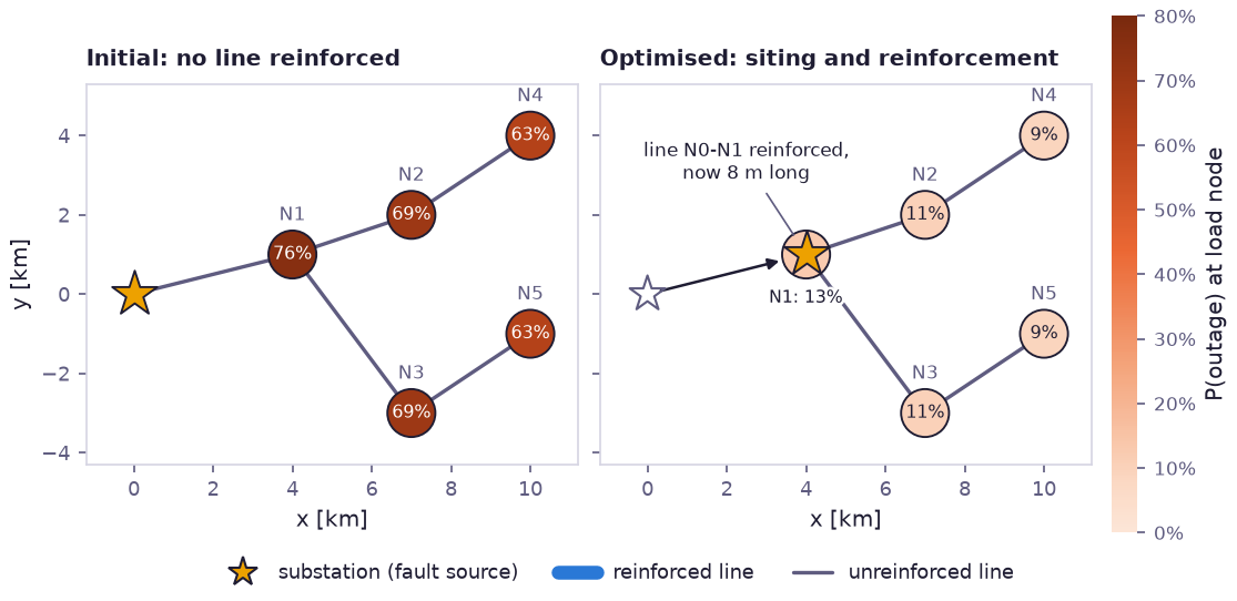
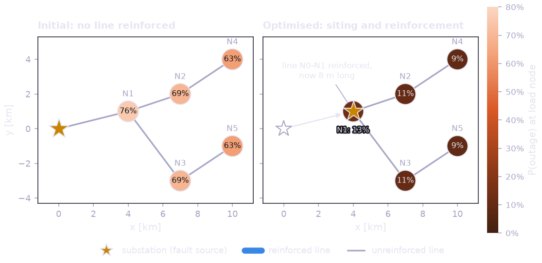
The feeder before and after the joint optimisation. Load nodes are coloured and labelled by their outage probability, marginalised over the Weibull fault severity, for the hard (0/1) designs. Left: with no line reinforced, a substation fault reaches every node and 63 to 76 % of them lose supply. Right: the optimiser reinforces the line out of the substation and moves the substation onto node N1 (arrow). A fault is then contained at its source, and the outage probabilities fall to 9 to 13 %. Because reinforcement cost is proportional to line length and the reinforced line shrinks to 8 m, the reinforcement is almost free. Only the cost term links the substation site to the objective.

Step 1 — The network

Nodes are a PointList in a shared frame; edges are a fixed (m, 2) connectivity array. The substation’s position is a Param — siting is a design variable — while the load nodes stay fixed.

import jax.numpy as jnp
import prophys as prp

site = prp.Frame("site", units="km")

substation = prp.Param("substation_pos", shape=(2,), init=jnp.array([0.0, 0.0]))
loads = jnp.array([[4.0, 1.0], [7.0, 2.0], [7.0, -3.0], [10.0, 4.0], [10.0, -1.0]])
nodes = prp.stack([substation, *[loads[i] for i in range(loads.shape[0])]], axis=0)
edges = jnp.array([[0, 1], [1, 2], [1, 3], [2, 4], [3, 5]])
grid = prp.Network(nodes, edges, site)

grid.edge_lengths()     # (5,), differentiable in substation_pos
grid.total_length()     # scalar, e.g. a cabling-cost proxy

Step 2 — Reinforcement as a differentiable decision

Whether each line is reinforced is naturally binary, but it needs a gradient to be optimized alongside the continuous siting variable. A BinaryState per edge does exactly that: it evaluates to a hard 0/1 in eval mode and a smooth, temperature-relaxed value in opt mode, following the model’s compile(mode=, tau=) setting like every other primitive in the library.

reinforced = prp.stack(
    [prp.BinaryState(f"reinforce_{i}", init=0.3) for i in range(edges.shape[0])], axis=0
)
# A reinforced line contains 90% of an incoming fault; an unreinforced
# line passes 80% of it downstream.
transmission = 0.8 - 0.7 * reinforced

Step 3 — Cascading a fault along the network

Network.propagate runs a K-hop linear cascade of a per-node signal along the directed edges, scaled by the per-edge transmission weight at every hop — a fault injected at the substation decays as it crosses reinforced lines and persists across unreinforced ones:

fault_severity = prp.RandomVariable("fault_severity", prp.Weibull(scale=1.0, concentration=1.5))

def cascade_load_loss(severity):
    unit_fault = jnp.zeros(grid.n_nodes).at[0].set(1.0)
    response = grid.propagate(unit_fault, steps=3, weights=transmission)  # (n_nodes,)
    return severity[..., None] * response

load_at_risk = cascade_load_loss(fault_severity)  # (6,), stochastic

The cascade is linear in its source, so a unit fault is propagated once through the network and scaled by the severity. [..., None] broadcasts the severity against the node axis, so the same expression serves a single design-point severity and a batch of Monte Carlo draws.

This is entirely differentiable in both the node coordinates (via edge_lengths/geometry feeding the cost term below) and the per-edge weights — with BinaryState weights, the cascade topology itself becomes a design variable.

Step 4 — Outage risk and reinforcement cost

Each load node’s outage probability is a smoothed threshold on the fraction of load at risk; reinforcement has a cost proportional to line length, charged only for lines actually reinforced:

outage_prob = prp.clip(prp.sigmoid(10.0 * (load_at_risk[..., 1:] - 0.3)), 1e-4, 1 - 1e-4)
outage_events = [
    prp.UncertainAttribute(f"outage_node_{i + 1}", prp.Bernoulli(prob=outage_prob[..., i]))
    for i in range(loads.shape[0])
]
model = prp.ProbabilityModel(*outage_events)

line_cost = grid.edge_lengths() * 50.0
reinforcement_cost = prp.sum_(line_cost * reinforced)

Note the ... in load_at_risk[..., 1:]: once fault_severity is marginalized over Monte-Carlo samples, load_at_risk carries a leading sample axis — plain [1:] would slice that axis instead of the node axis. This is the same broadcasting discipline covered in Marginalizing over random inputs.

Step 5 — Joint design optimization

A single optimize() call minimizes expected outage risk plus reinforcement cost with respect to both the relaxed reinforcement decisions and the substation site:

objective = (
    prp.sum_(prp.stack([outage_prob[..., i] for i in range(loads.shape[0])], axis=0))
    + 0.01 * reinforcement_cost
)
reinforce_params = [p for p in model.params().values() if p.name.startswith("reinforce_")]
result = prp.optimize(
    objective,
    wrt=[*reinforce_params, substation],
    n_steps=200,
    learning_rate=0.1,
    extra_env={"fault_severity": 1.0, "__mode__": "opt", "__tau__": 3.0},
)

The optimizer trades off which lines are worth reinforcing against where the substation sits. This joint discrete/continuous decision would otherwise need a mixed-integer solver; here plain gradient descent resolves it.

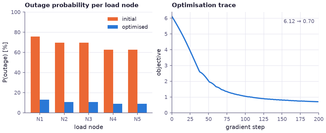
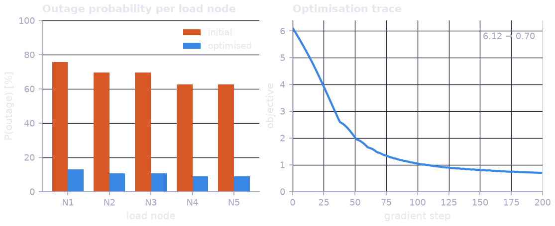
Left: outage probability per load node for the initial and the optimised design. The reduction is largest at N1, next to the fault source. Right: the objective (summed outage probability at full fault severity, plus the reinforcement cost) over 200 Adam steps. It falls from 6.1 to 0.7 as the relaxed decision on the first line saturates at “reinforced” and the decisions on the other lines go to “not reinforced”.

Results

=== Forward model (deterministic snapshot, full-severity fault) ===
edge lengths (km): [4.1231055 3.1622777 5.        3.6055512 3.6055512]
load at risk per node: [1.         0.8        0.64000005 0.64000005 0.512      0.512     ]
reinforcement cost (initial): 0.0
P(outage_node_1) = 0.616723
P(outage_node_2) = 0.36345038
P(outage_node_3) = 0.36345038
P(outage_node_4) = 0.16429265
P(outage_node_5) = 0.16429265

=== Design optimization ===
initial objective: 6.115460395812988
final objective: 0.6967688798904419
reinforcement decisions (relaxed): {'reinforce_0': Array(10.799474, dtype=float32), 'reinforce_1': Array(-12.943474, dtype=float32), 'reinforce_2': Array(-12.221089, dtype=float32), 'reinforce_3': Array(-11.59827, dtype=float32), 'reinforce_4': Array(-11.598477, dtype=float32)}
optimized substation site: [4.00591   1.0051738]

=== Export ===
exported attributes: ['outage_node_1', 'outage_node_2', 'outage_node_3', 'outage_node_4', 'outage_node_5']

The relaxed reinforcement decisions are printed as raw BinaryState logits: a large positive value means “reinforce” and a large negative one “do not”. The outage probabilities printed at the top come from the model compiled in opt mode, where the initial decisions are relaxed to about 0.43. The figures use the hard 0/1 designs (eval mode), which is why their initial values are higher.

Running it

$ python examples/electric_grid/model.py