Transformations

A Transform is a composable, callable mapping Expr -> Expr. Bijective transforms additionally implement inverse and log_det_jacobian, so they can double as a distribution bijector via TransformedDistribution.

Linear

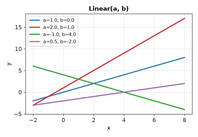
a * x + b — bijective, with closed-form inverse.

Affine

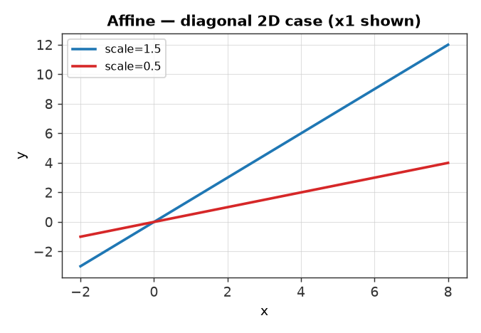
A @ x + b for vector-valued x.

Polynomial

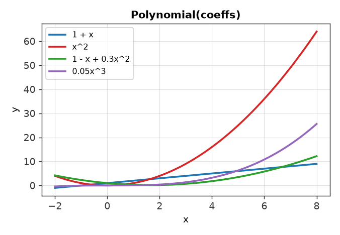
sum_i coeffs[i] * x**i.

PiecewiseLinear

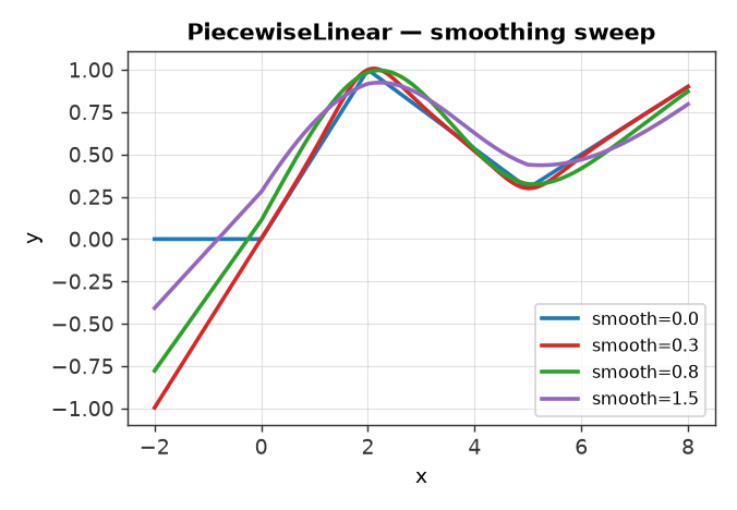
smooth=0 gives the exact (subgradient) curve; smooth=tau blends neighbouring segments for a fully continuous gradient at the knots.

Decay

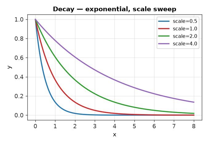
Exponential (exp(-x/scale)) or power-law decay, typically composed after a distance primitive.

Logistic

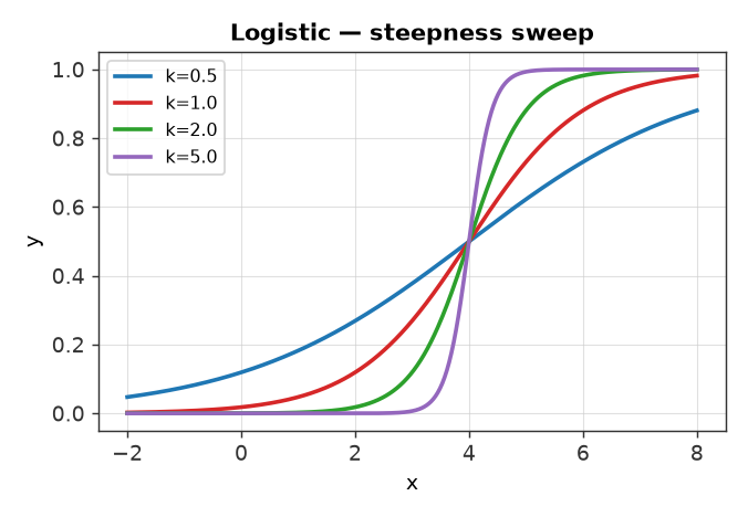
Dose-response / regulatory-acceptance curves.

TableLookup1D

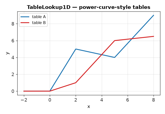
Interpolated 1D characteristic curve (e.g. a power curve).

TableLookup2D

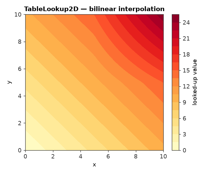
Bilinearly interpolated 2D lookup (e.g. sound power level over wind speed x direction).

Smoothing behavior of PiecewiseLinear

Because a hard piecewise-linear kink has a discontinuous gradient at each knot, PiecewiseLinear lets the smoothing temperature trade exactness against gradient continuity:

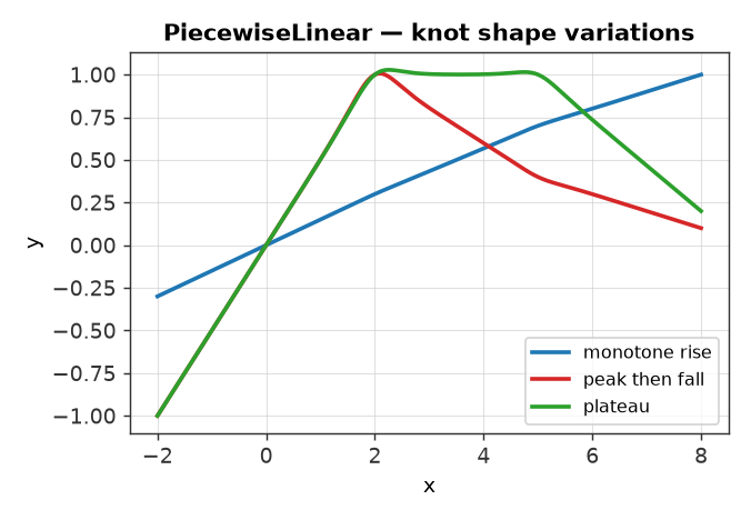
A smooth value that is too large relative to the knot spacing will blend in neighbouring segments’ slopes even at points deep inside one segment — worth checking for if a transformed probability unexpectedly drifts outside its valid range (e.g. below 0 for a probability fed into Bernoulli).

class prophys.transformations.Transform

Base class for symbolic transformations.

Subclasses implement __call__. Bijective transforms additionally implement inverse and log_det_jacobian so they can be used to build a TransformedDistribution.

then(other)

Compose: self.then(other)(x) == other(self(x)).

Parameters:

other (Transform)

Return type:

Transform

class prophys.transformations.Linear(a=1.0, b=0.0)

y = a * x + b (scalars or broadcastable arrays; a, b may be Expr, e.g. Param, making the slope/intercept learnable).

Parameters:

• a (Any)

• b (Any)

class prophys.transformations.Affine(A, b=0.0)

y = A @ x + b for vector-valued x.

Parameters:

• A (Any)

• b (Any)

class prophys.transformations.Polynomial(coeffs)

y = sum_i coeffs[i] * x**i (coeffs may contain Expr values).

Parameters:

coeffs (Sequence[Any])

class prophys.transformations.PiecewiseLinear(knots, values, smooth=0.0)

A piecewise-linear curve through (knots[i], values[i]), clamped flat beyond the endpoints.

smooth=0 (default) gives the exact, subgradient-valid PWL function (matches e.g. a dose-response table exactly). smooth=tau > 0 uses a soft segment-blend so the gradient is continuous across knots too, useful when knot locations themselves are being optimized.

Parameters:

• knots (Sequence[float])

• values (Sequence[float])

• smooth (float)

class prophys.transformations.Decay(scale=1.0, kind='exp')

Exponential (exp(-x/scale)) or power-law (x**(-p)) decay, typically composed after a distance primitive.

Parameters:

• scale (Any)

• kind (str)

class prophys.transformations.Logistic(x0=0.0, k=1.0, L=1.0)

Dose-response curve: L / (1 + exp(-k * (x - x0))).

Parameters:

• x0 (Any)

• k (Any)

• L (Any)

class prophys.transformations.TableLookup1D(grid, values)

Interpolated 1D lookup table (alias for PiecewiseLinear under a more descriptive name for physical characteristic curves, e.g. a wind turbine power curve).

Parameters:

• grid (Sequence[float])

• values (Sequence[float])

class prophys.transformations.TableLookup2D(x_grid, y_grid, values)

Bilinearly interpolated 2D lookup table, e.g. sound power level as a function of (wind speed, wind direction).

Parameters:

• x_grid (Sequence[float])

• y_grid (Sequence[float])

• values (Sequence[Sequence[float]])

Periodic & recurring phenomena

For seasonal, diurnal, tidal, or otherwise recurring signals — and for the “return period” framing common in extreme-event risk (e.g. a “100-year flood”).

class prophys.transformations.Phase(period=1.0)

Wrap a continuous variable (e.g. elapsed time) into [0, period), e.g. turning “hours since start” into “hour of day”.

Uses floor-modulo, which is continuous except at the wrap points (measure zero) — the same character as the library’s other hard boundary primitives (PiecewiseLinear with smooth=0, polygon containment).

Parameters:

period (Any)

class prophys.transformations.Periodic(period, amplitude, phase=None, offset=0.0)

A learnable finite Fourier series: the standard, fully differentiable building block for seasonal/diurnal/tidal signals.

y = offset + sum_k amplitude[k] * cos(2*pi*k*x/period - phase[k])

amplitude and phase are sequences of per-harmonic coefficients (length = number of harmonics); all may be Expr (typically Param), so the shape of a seasonal cycle can be learned from data via the same fit_distribution/calibrate/finetune machinery used elsewhere.

Parameters:

• period (Any)

• amplitude (Sequence[Any])

• phase (Sequence[Any] | None)

• offset (Any)

class prophys.transformations.ReturnPeriod

Convert an annual exceedance probability to a return period (the familiar “100-year flood” framing) and back.

return_period = 1 / exceedance_probability

Bijective and defined for p in (0, 1]; use inverse to go from a target return period back to the probability a per-event/per-year model needs to reproduce it.

class prophys.transformations.RecurrenceRate

Convert a mean inter-event time (period) to an event rate, the natural parameter for a Poisson process modeling recurring hazards (equipment failures, extreme-weather events, …).

rate = 1 / mean_interval, composable with Periodic (a time-varying rate) to build a non-homogeneous Poisson process: sample counts over a window via prp.Poisson(rate_transform(t_window)).