

Example: Fatigue of a Railway Bridge Detail#
A single-track line crosses a river on a 15 m simply supported steel plate-girder bridge. Transverse web stiffeners are welded to the girders every metre, and the weld toe at the tension flange is a fatigue detail of category 80 (EN 1993-1-9). The owner asks how quickly the traffic consumes the fatigue life of the midspan detail, when the first inspection is due, and how thick the tension flange would have to be for the detail to last its 100-year service life without relying on inspection.
The model simulates every passage from first principles: axle loads move over
the span, the bending stress at each stiffener follows from influence lines,
the stress history of every train is rainflow counted and summed by the
Palmgren–Miner rule with fatigue_damage(), and a whole
day of mixed traffic is one Monte Carlo sample. Strain-gauge records calibrate
the load share of the girder, freight traffic grows along a random path
(RandomWalk), and the flange is designed by gradient descent
through the rainflow counting itself. The full runnable source is
examples/rail_fatigue/model.py.
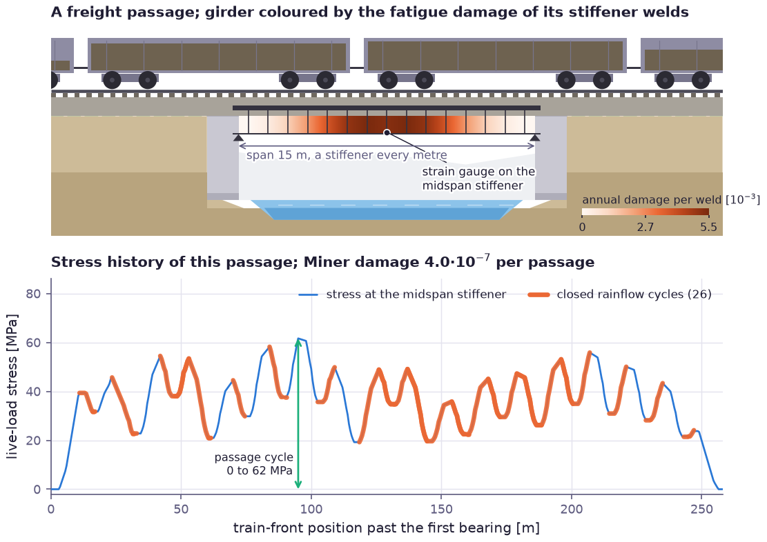
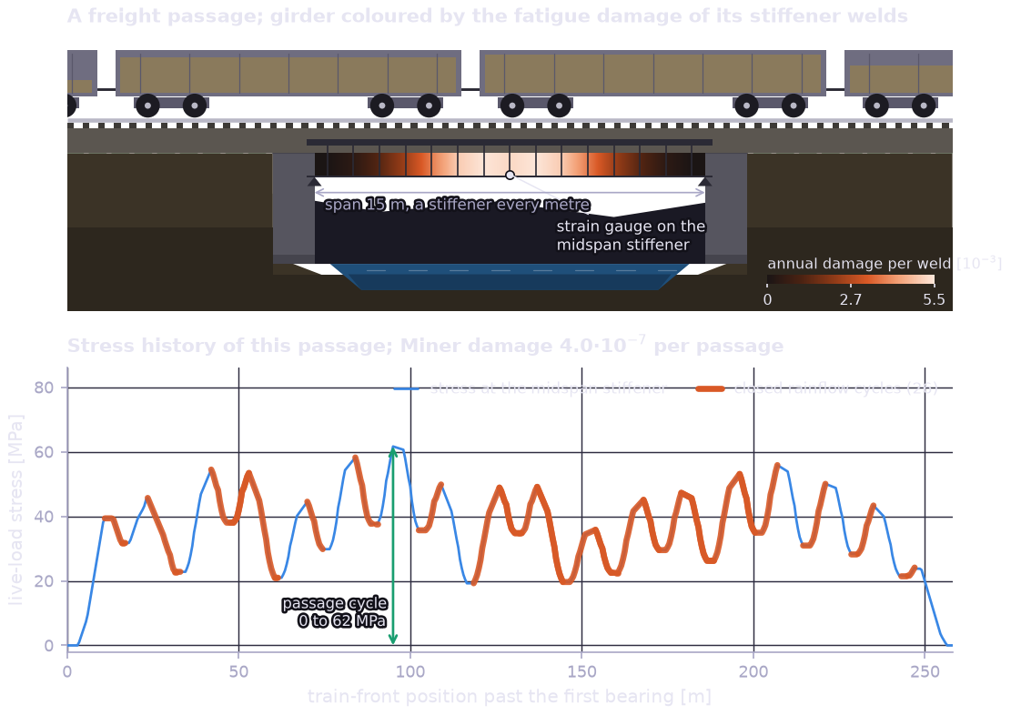
Top: the most damaging freight passage of a simulated day, drawn at the position where the midspan stress peaks; each open wagon is filled to its own sampled payload. The girder web is coloured by the annual Miner damage of the stiffener welds along the span, which concentrates at midspan where the moment influence line is largest. Bottom: the stress history of that passage at the instrumented midspan stiffener. The orange segments are the 26 closed rainflow cycles, one or two per wagon; the green arrow is the passage cycle from zero to the peak and back, counted as two half cycles.
Step 1 — The girder and the detail#
The girder is a welded I-section whose flange thickness is the design
variable. The detail uses the EN 1993-1-9 category 80 curve with a single
slope m = 3 and no constant-amplitude fatigue limit, the conservative form
of the curve:
WEB_DEPTH, WEB_T, FLANGE_B = 1.20, 0.012, 0.40  # welded I-girder [m]
flange_t = prp.Param("flange_t", init=0.030)  # flange thickness [m], the design variable


def section_modulus(t_f):
    """Elastic section modulus of the doubly symmetric I-girder [m^3]."""
    inertia = WEB_T * WEB_DEPTH**3 / 12.0 + 2.0 * FLANGE_B * t_f * (WEB_DEPTH / 2.0 + t_f / 2.0) ** 2
    return inertia / (WEB_DEPTH / 2.0 + t_f)


# EN 1993-1-9 detail category 80: N = 2e6 (80 / S)^3. A single slope m = 3,
# without the constant-amplitude fatigue limit, is the conservative form.
SN_M = 3.0
DETAIL_CATEGORY = 80.0  # [MPa]
K_CHAR = 2.0e6 * DETAIL_CATEGORY**SN_M  # characteristic S-N constant [MPa^3]
Step 2 — Trains and influence lines#
A freight train is a Bo’Bo’ locomotive and 16 four-axle wagons; a passenger
train is two four-car multiple units. The bending moment at a stiffener at
a from the bearing, for an axle at x on the span, is the influence
ordinate IL(x; a) = min(x (L - a), a (L - x)) / L. The ordinates for every
train position, axle and stiffener are fixed by geometry and computed once:
def influence_matrix(offsets, length):
    """Moment influence ordinates [m] at every stiffener, for every train
    position and axle: ``IL(x; a) = min(x (L - a), a (L - x)) / L`` on the
    span, zero off it. Shape ``(sections, positions, axles)``."""
    front = np.arange(0.0, length + SPAN + STEP, STEP)
    x = front[:, None] - offsets[None, :]  # axle positions on the bridge
    a = SECTIONS[:, None, None]
    return np.maximum(np.minimum(x * (SPAN - a), a * (SPAN - x)), 0.0) / SPAN
Step 3 — A day of traffic as one Monte Carlo sample#
The payload of every wagon of the day’s 24 freight trains, the occupancy of
every car of the 60 passenger trains, and the dynamic amplification of every
passage (EN 1991-2 Annex D gives phi = 1.08 for this span and speed) are
random inputs. They are vector-valued random variables whose leading axis of
length one is the Monte Carlo sample axis, so every sample draws a complete day:
payload = prp.RandomVariable(  # payload fraction of every wagon of every freight train of the day
    "payload", prp.Uniform(jnp.full((1, FREIGHT_PER_DAY, N_WAGONS), 0.3), 1.0)
)
occupancy = prp.RandomVariable(  # occupancy of every passenger car
    "occupancy", prp.Uniform(jnp.zeros((1, PASSENGER_PER_DAY, N_CARS)), 1.0)
)
# Dynamic amplification per passage. EN 1991-2 Annex D for L = 15 m,
# n0 = 8 Hz, v = 100 km/h: phi = 1 + (phi' + phi''/2)/2 = 1.08.
daf_freight = prp.RandomVariable(
    "daf_freight", prp.LogNormal(jnp.full((1, FREIGHT_PER_DAY), jnp.log(1.08)), 0.04)
)
The stress history of a passage superposes the axle loads on the influence
ordinates and scales by the dynamic factor, the girder’s share of the track
load and the section modulus. The load share is a bounded
Param, 0.5 by the design assumption:
load_share = prp.Param("load_share", init=0.5, bounds=(0.2, 0.8))


def stress_history(axle_loads, daf, il):
    """Bending stress [MPa] at a stiffener while a train crosses,
    ``sigma = phi * share * sum_a P_a IL(x_a) / W``. With ``il`` of shape
    ``(positions, axles)`` the result is ``(..., trains, positions)``; with
    ``(sections, positions, axles)`` it is ``(..., trains, sections, positions)``."""
    pattern = "...a,pa->...p" if il.ndim == 2 else "...a,spa->...sp"
    moment = op("influence_superposition", lambda p: jnp.einsum(pattern, p, il), axle_loads)  # [kNm]
    per_train = op("per_train", lambda d: d.reshape(d.shape + (1,) * (il.ndim - 1)), daf)
    return moment * per_train * (load_share / section_modulus(flange_t) / 1000.0)  # kNm / m^3 -> MPa
Step 4 — Rainflow counting and Miner damage#
fatigue_damage() counts the cycles of every history by
the rainflow method (ASTM E1049) and sums n S^m / K over them. Welded
details are insensitive to the mean stress, so no Goodman correction is
applied. The histories of all trains of all sampled days go in as one
[batch, T] block:
def miner_damage(history):
    """Rainflow-counted Palmgren-Miner damage of every stress history ``(..., T)`` -> ``(...)``,
    on the characteristic S-N curve. The histories are passed as one ``[batch, T]`` block."""
    flat = op("flatten_histories", lambda s: s.reshape(-1, s.shape[-1]), history)
    damage = physics.fatigue_damage(flat, sn_exponent=SN_M, sn_coefficient=K_CHAR)
    return op("restore_batch", lambda d, s: d.reshape(s.shape[:-1]), damage, history)


damage_freight = miner_damage(sigma_freight)  # (..., 24) per freight passage
damage_passenger = miner_damage(sigma_passenger)  # (..., 60) per passenger passage
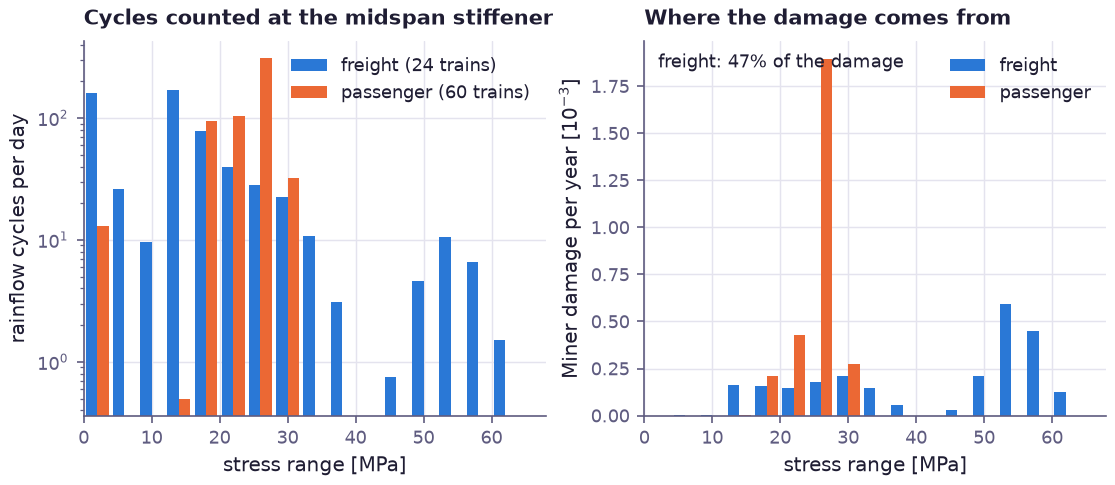
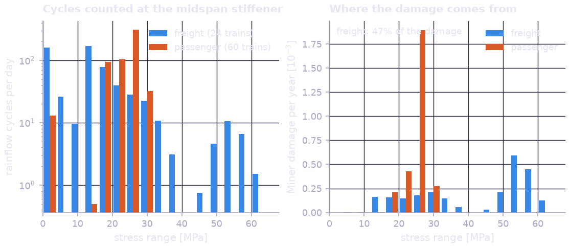
Rainflow cycles per day at the midspan stiffener by stress range (left, log scale) and the annual damage they cause (right), from eight simulated days. Freight trains produce the few large cycles of 45 to 65 MPa, one per passage, while the passenger cars produce hundreds of cycles near 27 MPa. With the cube law both matter: passenger traffic causes about half of the damage, so neither train type can be dropped from the assessment.
Step 5 — Calibrating the load share to strain-gauge records#
A strain gauge on the midspan stiffener recorded the peak stress of 120 freight
passages. The peak of a passage is an
UncertainAttribute whose mean is the model’s peak
stress, marginalized over the payloads and the dynamic factor of the passage.
calibrate() fits the load share and the gauge noise by
maximum likelihood, and parameter_uncertainty() gives
their standard errors:
peak_stress = prp.UncertainAttribute(
    "peak_stress",
    prp.Gaussian(mean=op("time_max", lambda s: jnp.max(s, axis=-1), gauge_history), sigma=gauge_sigma),
    unit="MPa",
    domain="peak live-load stress at the midspan stiffener during a freight passage",
)
...
cal = prp.calibrate(
    compiled, "peak_stress", records, trainable=["load_share", "gauge_sigma"], n_steps=150, learning_rate=0.2
)
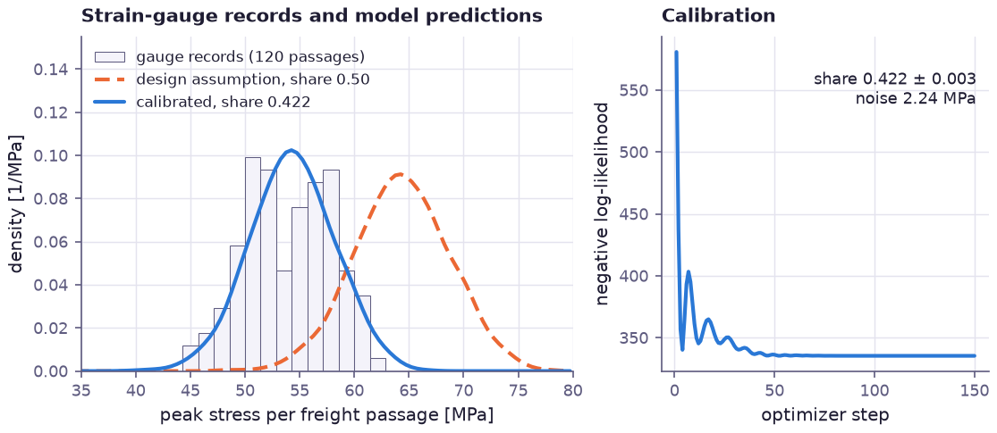
The measured peaks (histogram) lie well below the prediction of the design assumption of an equal split between the two girders (dashed): the deck and the bracing spread the load, and the instrumented girder carries 42 % of it. With a cubic S–N curve that 16 % reduction of stress lowers the damage by 40 %, which is why the monitoring campaign pays for itself. Right: the calibration converges in about 50 steps.
Step 6 — Service life: traffic growth and resistance#
Freight volume grows along an uncertain path, a random walk of its logarithm with a drift of 1 % a year. Each year adds the day’s damage times 365 and the growth factor, and the Miner sum accumulates:
freight_growth = prp.RandomVariable(  # log of the freight volume relative to today
    "freight_growth", prp.RandomWalk(init=0.0, innovation=prp.Gaussian(0.01, 0.025), n_steps=YEARS)
)
freight_daily = prp.sum_(damage_freight, axis=-1)
passenger_daily = prp.sum_(damage_passenger, axis=-1)
annual = 365.0 * (prp.processes.over_time(freight_daily) * prp.exp(freight_growth)
                  + prp.processes.over_time(passenger_daily))  # (..., years)
cumulative = op("cumsum", lambda d: jnp.cumsum(d, axis=-1), annual)  # Miner sum, characteristic curve
The resistance combines the Miner sum at failure (lognormal, median 1,
coefficient of variation 0.3, JCSS), the S–N scatter (standard deviation 0.2
of log10 N, the characteristic curve lying two standard deviations below
the mean) and a stress model factor (lognormal, 8 %). All three are lognormal,
so given a traffic draw the probability that the detail has failed by year
t is an exact normal probability,
Phi((ln D(t) - mu_R) / sigma_R), evaluated with
ndtr(). Averaging it over the traffic draws is the
expectation of a path-valued Bernoulli attribute:
# Failure by year t: P(ln D(t) > ln R) = Phi((ln D(t) - mu_R) / sigma_R), exact given the traffic draw.
pf_given_traffic = prp.symbolic.ndtr((prp.log(cumulative) - MU_R) / SIGMA_R)
fatigue_failure = prp.UncertainAttribute(
    "fatigue_failure", prp.Bernoulli(prob=pf_given_traffic), domain="fatigue failure of the detail by each year"
)
...
pf = np.asarray(compiled.expectation("fatigue_failure", params=params))  # one value per year
Conditioning on the traffic and integrating the resistance exactly is what
makes failure probabilities of order 1e-5 accurate with a few hundred
samples.
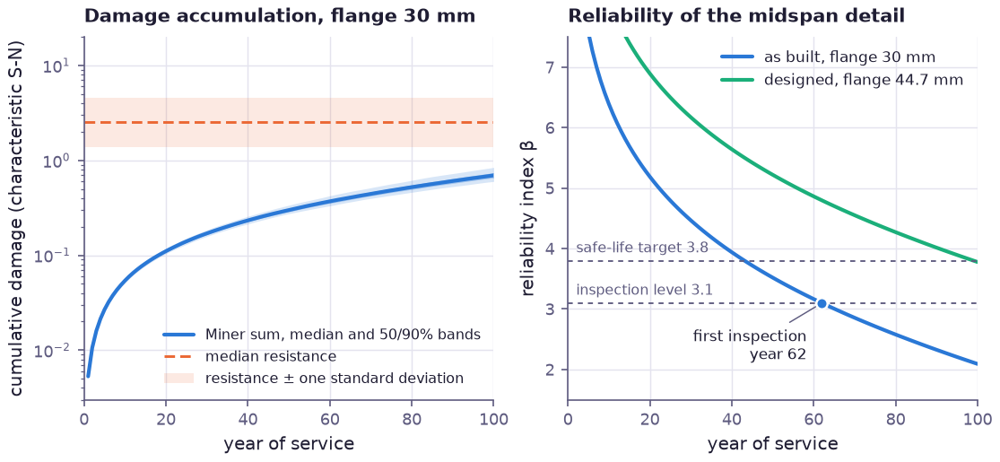
Left: the Miner sum on the characteristic curve grows almost linearly with a slight upward bend from traffic growth; its 50 % and 90 % bands from the traffic path are narrow next to the scatter of the resistance (shaded), which dominates the reliability. Right: the reliability index of the midspan detail falls below the safe-life target of 3.8 in year 44 and reaches the inspection level of 3.1 in year 62, when the first inspection is due. The designed flange stays above the target until the end of the service life, where it reaches 3.78 (the shortfall of 0.02 is the tolerance of the quadratic constraint penalty).
Step 7 — Designing the flange by gradient descent#
The lightest flange that meets the safe-life target is found by
optimize(): minimize the thickness subject to the
probability of failure by year 100 staying below Phi(-3.8). The failure
probability is a sample average over 128 common traffic draws, and its
gradient with respect to the flange thickness flows through the section
modulus, the stress histories and the rainflow counting:
draws = traffic_draws(128, seed=3)
pf_100 = prp.mean(pf_given_traffic[..., -1])
target = float(prp.Gaussian(0.0, 1.0).cdf(jnp.asarray(-BETA_SAFE_LIFE)).evaluate({}))
result = prp.optimize(
    flange_t * 1000.0,  # flange thickness [mm], proportional to the steel mass
    wrt=[flange_t],
    constraints=[prp.log(pf_100) - float(np.log(target))],
    penalty_weight=20.0,
    n_steps=200,
    learning_rate=0.0005,
    extra_env={**draws, "load_share": params["load_share"]},
)
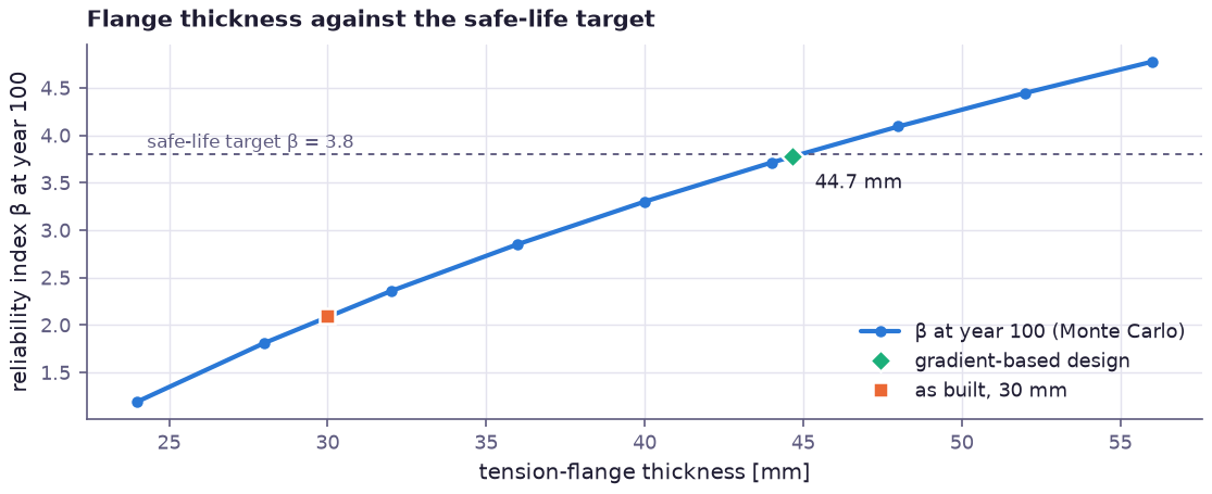
The reliability index at year 100, evaluated by the compiled model for a range of flange thicknesses, against the safe-life target. The as-built 30 mm flange reaches β = 2.1; the gradient-based design lands on the target at 44.7 mm without a grid search. Each extra millimetre of flange buys about 0.1 of reliability index here.
Results#
=== Calibration to strain-gauge records ===
  records: 120 freight passages, mean peak 54.0 MPa
  load share: 0.422 +/- 0.003 (design assumption 0.500)
  gauge noise: 2.24 MPa

=== Damage at the midspan stiffener (calibrated, flange 30 mm) ===
  first-year damage: median 5.22e-03, 90% interval [3.46e-03, 7.70e-03]
  CVaR95 first-year damage: 8.62e-03
  P(failure by year 50)  = 2.16e-04  (beta 3.52)
  P(failure by year 100) = 1.82e-02  (beta 2.09, safe-life target 3.8)
  first inspection (beta < 3.1): year 62

=== Design of the tension flange ===
  safe-life flange thickness: 44.7 mm (was 30.0 mm)
  beta at year 100: 3.78
The as-built detail is adequate as a damage-tolerant detail with a first inspection in year 62, but not as a safe-life detail; a 44.7 mm flange would make it one.
Primitives exercised#
Feature |
Used for |
|---|---|
Rainflow counting and Palmgren–Miner damage of every passage, with gradients to the stress histories |
|
|
Wagon payloads, car occupancy and dynamic amplification, a whole day of traffic per sample |
Uncertain growth of the freight volume over the service life |
|
Exact failure probability given the traffic, for every year |
|
Girder load share from strain-gauge records, with its standard error |
|
|
Failure probability per year, damage quantiles and tail |
Flange thickness against the reliability target |
Running it#
$ python examples/rail_fatigue/model.py
The model runs in about 15 seconds on a laptop CPU.