

Example: Well Field Beside a Protected Fen#
A water utility must deliver 60 l/s through the six-month dry season from four wells in an unconfined sand-and-gravel aquifer beside a river. A protected fen lies 1.2 km north of the well field, and its permit caps the dry-season lowering of the water table beneath it at 0.25 m, to be met with 95 % probability. The aquifer is known only from a three-day pumping test. How should the demand be split between the wells so that the permit holds at the least pumping power?
The drawdown is the Theis solution, evaluated by
superpose() with its radial E1 kernel, and the river
enters exactly through image wells. The model calibrates transmissivity and
specific yield to the pumping test with calibrate(),
turns the fit’s curvature into a correlated posterior with
parameter_uncertainty(), marginalizes it to obtain the
distribution of the fen drawdown and the probability of a permit breach, and
chooses the split of the demand with optimize() under a
chance constraint. The full runnable source is
examples/groundwater_wells/model.py.
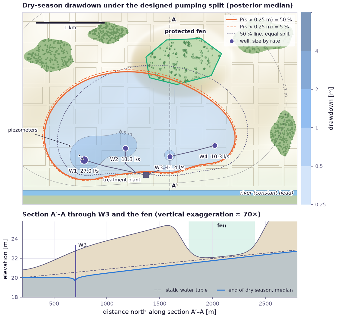
Top: the posterior-median drawdown at the end of the dry season under the designed split, over the site (the terrain, fields and woods are scenery). The river holds the water table, so the cone of depression is cut off to the south and stretches north towards the fen. The orange lines bound where the drawdown exceeds 0.25 m with 50 % and 5 % probability; the dotted line is the 50 % line of an equal split, which reaches into the fen. Wells are sized by their designed rate; the triangles are the piezometers of the pumping test. Bottom: section A′–A through W3 and the fen, with the static water table and the median water table at the end of the season. The fen sits in a hollow where the ground meets the water table, which is why a few decimetres of drawdown matter.
Step 1 — Theis drawdown with a river boundary#
For a well pumping Q from an aquifer of transmissivity T and
storativity (for an unconfined aquifer, specific yield) S, the drawdown at
distance r after a time t is s = Q / (4 pi T) W(u) with
u = r^2 S / (4 T t) and the Theis well function W = E1. The
radial_exp1 kernel of superpose() sums
strength * E1(r^2 / radial_scale) over sources, so the Theis solution is a
single call with radial_scale = 4 T t / S. The river bank is a
constant-head line; mirroring each pumping well across it as an injecting
image well makes the drawdown vanish on the bank exactly:
def drawdown(receptors, rates, log_t, log_s, time):
    """Drawdown [m] at `receptors` after pumping `rates` [m^3/s] for `time` [s].

    Theis (1935): s = sum_i Q_i / (4 pi T) [W(u_i) - W(u_i')], u = r^2 S / (4 T t),
    with u_i' measured from the image of well i across the river. `log_t`
    (transmissivity [m^2/s]) and `log_s` (storativity or specific yield [-]) may carry a
    leading Monte Carlo axis; the result is ``[..., receptors]``."""
    transmissivity, storativity = prp.exp(log_t), prp.exp(log_s)
    sources = np.vstack([xyz(WELLS), xyz(image(WELLS))])
    strengths = prp.symbolic.concatenate([rates, -rates], axis=-1)
    well_function_sum = physics.superpose(
        xyz(receptors), sources, strengths, kind="radial_exp1",
        radial_scale=4.0 * transmissivity * time / storativity,
    )
    per_receptor = op("per_receptor", lambda v: jnp.asarray(v)[..., None], transmissivity)  # (...,) -> (..., 1)
    return well_function_sum / (4.0 * jnp.pi * per_receptor)
The aquifer parameters enter in logarithms, so they stay positive under any gradient step and their posterior is close to Gaussian.
Step 2 — Calibrating to the pumping test#
W1 pumped 25 l/s for 72 hours while loggers in three piezometers, 30, 100 and
300 m away, recorded the drawdown fourteen times each. The 42 readings are one
vector-valued UncertainAttribute with the logger
accuracy of 1.5 cm, and the calibration starts from a prior guess based on the
grain size:
log_T = prp.Param("log_T", init=float(np.log(5e-3)))  # prior guess from grain size: T = 5e-3 m^2/s
log_S = prp.Param("log_S", init=float(np.log(0.2)))  # specific yield of the unconfined aquifer
READING_SIGMA = 0.015  # logger accuracy incl. barometric effects [m]

test_rates = jnp.array([TEST_RATE, 0.0, 0.0, 0.0])
# One superpose call per reading time, concatenated to 14 times x 3 piezometers = 42 readings.
test_drawdown = prp.symbolic.concatenate(
    [drawdown(PIEZOMETERS, test_rates, log_T, log_S, t) for t in TEST_TIMES], axis=-1
)
test_readings = prp.UncertainAttribute(
    "test_readings",
    prp.Gaussian(mean=test_drawdown, sigma=READING_SIGMA),
    unit="m",
    domain="drawdown readings at the three piezometers during the pumping test",
)
calibrate() maximizes the likelihood, and
parameter_uncertainty() inverts the Hessian of the
negative log-likelihood at the optimum (the Laplace approximation). Its
covariance becomes the posterior of the aquifer, a
MultivariateGaussian random variable:
cal = prp.calibrate(compiled_test, "test_readings", readings[None, :], n_steps=300, learning_rate=0.1)
unc = prp.parameter_uncertainty(compiled_test, {"test_readings": readings[None, :]}, result=cal)
...
aquifer = prp.RandomVariable("aquifer", prp.MultivariateGaussian(posterior_mean, posterior_chol))
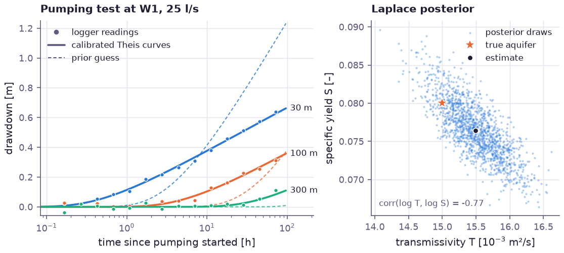
Left: the logger readings (dots), the Theis curves of the prior guess (dashed), which overpredict the drawdown near the well twofold, and the calibrated curves. Right: draws from the Laplace posterior. Transmissivity is known to 2.5 % and specific yield to 5 %, and the two are strongly negatively correlated (−0.77): a more transmissive and less storative aquifer produces nearly the same early drawdown. The aquifer that generated the synthetic readings (star) lies inside the posterior cloud.
Step 3 — The fen drawdown and its risk#
The permit applies to the mean drawdown over the fen, evaluated on a 75 m lattice of points inside its outline. Its distribution combines the posterior of the aquifer with a model error of 3 cm for the idealization of the aquifer as homogeneous. Given an aquifer draw, the probability of compliance is an exact normal probability, kept in logarithmic form so that its gradient never vanishes when the constraint is far from met:
aquifer = prp.RandomVariable("aquifer", prp.MultivariateGaussian(posterior_mean, posterior_chol))
fen = drawdown(FEN_POINTS, rates, aquifer[..., 0], aquifer[..., 1], DRY_SEASON)
fen_mean = prp.mean(fen, axis=-1)
fen_drawdown = prp.UncertainAttribute(
    "fen_drawdown",
    prp.Gaussian(mean=fen_mean, sigma=MODEL_ERROR),
    unit="m",
    domain="mean dry-season drawdown beneath the fen",
)
# Exact compliance probability given the aquifer draw, in log form so that
# its gradient never vanishes: log P(s <= L) = log Phi((L - s_mean) / sigma).
log_comply = prp.symbolic.log_ndtr((FEN_LIMIT - fen_mean) / MODEL_ERROR)
The compiled model reports the expectation, the 95 % quantile and the CVaR of
the fen drawdown, and the breach probability 1 - E[F(0.25 | aquifer)]
from its conditional CDF, which carries no sampling noise from the model
error.
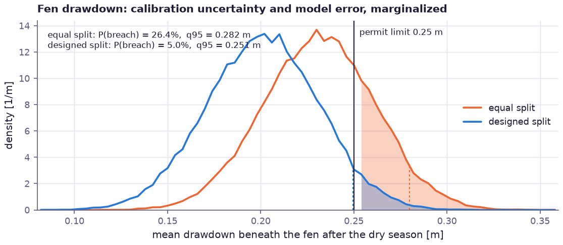
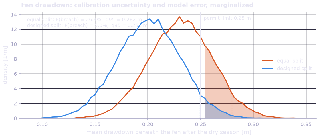
Distribution of the mean fen drawdown at the end of the dry season for an equal split of the demand and for the designed split, with the part beyond the permit limit shaded and the 95 % quantiles marked (dotted). Splitting the demand equally breaches the permit with a probability of 26 %; the designed split shifts the distribution by 3 cm and brings the probability to 5.0 %, with the 95 % quantile on the limit.
Step 4 — Splitting the demand at least power#
The split is a normalized exponential of four free logits, so the rates always
add up to the demand. The pumping power counts the static lift, the aquifer
drawdown at each well (its own cone and the interference of the others) and
the Jacob well loss C Q^2:
split = [prp.Param(f"split_{name}", init=0.0) for name in WELL_NAMES]
weights = prp.exp(prp.stack(split, axis=0))
rates_ls = DEMAND * weights / prp.sum_(weights)  # [l/s]
rates = rates_ls / 1000.0  # [m^3/s]
...
bores = WELLS + np.array([WELL_RADIUS, 0.0])
lift = STATIC_LIFT + prp.mean(drawdown(bores, rates, aquifer[..., 0], aquifer[..., 1], DRY_SEASON), axis=0)
power = 9.81 * prp.sum_(rates * (lift + WELL_LOSS * rates**2)) / PUMP_EFFICIENCY
The design minimizes the power subject to a compliance probability of at least 95 %, averaged over 256 posterior draws, and to the pump capacities:
log_p_comply = prp.symbolic.logsumexp(log_comply) - float(np.log(n_draws))
constraints = [float(np.log(0.95)) - log_p_comply, rates_ls - MAX_RATE]
result = prp.optimize(
    power, wrt=split, constraints=constraints, penalty_weight=1e4,
    n_steps=300, learning_rate=0.1, extra_env={"aquifer": draws},
)
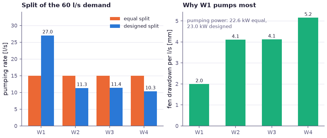
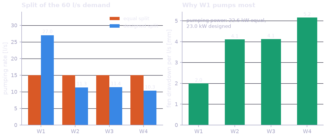
Left: the equal split and the designed split of the 60 l/s demand. Right: the mean fen drawdown per litre per second pumped at each well. W1 lies farthest from the fen and closest to the river, so each litre per second it pumps lowers the fen by 2 mm, against 4 to 5 mm for the other wells. The design moves pumping to W1 only as far as the permit requires, because concentrating the demand raises the drawdown and the well losses at W1 and with them the pumping power. Compliance costs 0.4 kW, under 2 % of the pumping power.
Results#
=== Pumping-test calibration (42 readings) ===
  T = 1.55e-02 m2/s  (sd of log T 0.025)
  S = 0.076          (sd of log S 0.048)
  corr(log T, log S) = -0.77

=== Dry season, demand 60 l/s (W1 W2 W3 W4) ===
  equal split: 15.0 15.0 15.0 15.0 l/s   power  22.6 kW
      fen: E[s]=0.231 m  q95=0.282 m  CVaR95=0.296 m  P(s > 0.25 m)=26.4%
  designed   : 27.0 11.3 11.4 10.3 l/s   power  23.0 kW
      fen: E[s]=0.201 m  q95=0.251 m  CVaR95=0.265 m  P(s > 0.25 m)=5.0%
Primitives exercised#
Feature |
Used for |
|---|---|
|
Theis drawdown of the wells and their river images at piezometers, fen points and well bores |
Transmissivity and specific yield from the pumping test, with their correlated Laplace posterior |
|
The posterior of the aquifer, marginalized by Monte Carlo |
|
|
Fen drawdown statistics and the exact breach probability |
The chance constraint in a form with non-vanishing gradients |
|
The split of the demand at least pumping power |
Running it#
$ python examples/groundwater_wells/model.py
The model runs in about 15 seconds on a laptop CPU.