Physics Primitives

prophys.physics holds generic building blocks for transport, dispersion, thermal, reliability and fatigue calculations. None of them is a model of a particular system: a Gaussian plume, a Theis drawdown or a wake deficit is a composition of a primitive with symbolic arithmetic. Every primitive returns an Expr, accepts constants, parameters, random variables or other expressions as arguments, and is backed by a native kernel with the same guarantees as the rest of prophys:

• Exact outputs. Closed forms, or finite algorithms whose step count is fixed or bounded by the size of the input — never a loop that runs “until converged”. Where a quantity is prone to cancellation or under/overflow (tail probabilities, large Poisson means, far polygon edges), the kernel evaluates it in a form that keeps its relative accuracy.

• Exact gradients with respect to every continuous argument.

• The same results on CPU and GPU: forward values bit for bit on the tested GPUs, gradients within a tight tolerance (see Kernel correctness).

Primitive	What it computes
erf(), erfcx(), log_ndtr(), exp1(), i0e() … owens_t()	Special functions for closed-form solutions (error functions far into the tails, the exponential integral, scaled Bessel functions, Owen’s T).
superpose()	Sums of anisotropic pair Green’s functions between sources and receptors: steady advected plumes, moving puffs, advancing fronts and radial E1 kernels, with power-law spreading, first-order decay and reflecting ground/lid images.
gaussian_polygon_probability()	Probability that a bivariate normal position falls in a polygon.
ray_integral()	Exact line integrals, maxima and threshold lengths of raster fields along segments.
propagate_linear()	The state of dx/dt = Q x + u after a time t (matrix exponential).
state_space_loglik()	The exact Kalman-filter log-likelihood of noisy observations.
overlap_area()	Intersection areas of polygons with polygons or disks.
piecewise_polynomial()	Published piecewise (log-)polynomial correlations from their coefficient tables.
network_potentials()	Potentials of grounded linear networks (DC power flow, resistor, heat and linearized pipe networks).
compound_distribution()	The exact pmf of aggregate losses or counts (Panjer’s recursion).
spectral_random_field()	Differentiable samples of stationary Gaussian random fields.
directional_sweep()	Node outputs under directional shadowing (wakes, sheltering).
fatigue_damage()	Rainflow-counted Palmgren–Miner damage of load histories.

Gallery of the primitives

Each figure below is computed by the primitive it shows, and the code under it sketches the call that produced it. Everything runs on the free tier.

Green’s functions: superpose

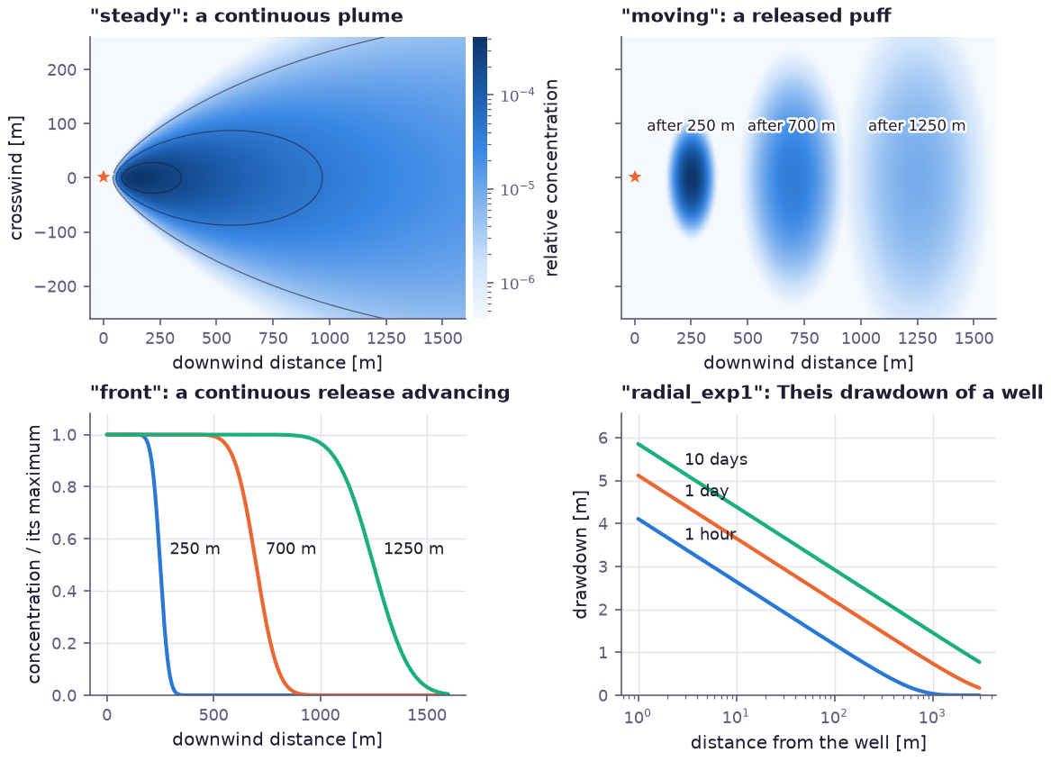
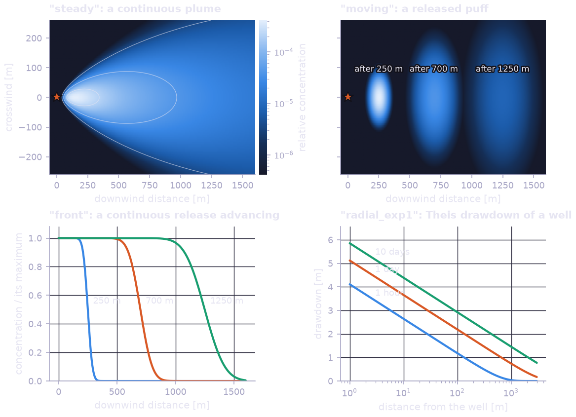
One primitive, four transport problems. Top: the ground-level concentration of a continuous release from a 20 m stack with a reflecting ground and an 800 m mixing lid, and a puff released from the same stack after it travelled 250, 700 and 1250 m. Bottom: the along-wind profile of a release that started at the stack and keeps going, and the Theis drawdown around a well pumping 20 l/s after an hour, a day and ten days.

plume = physics.superpose(receptors, stack, [1.0], kind="steady",
                          spread_across=(0.22, 0.9), spread_vertical=(0.2, 0.85),
                          vertical="reflect", lid=800.0, images=3)
puffs = physics.superpose(receptors, stack, [1.0], kind="moving",
                          travel=np.array([250.0, 700.0, 1250.0]), spread_along=(0.22, 0.9),
                          spread_across=(0.22, 0.9), spread_vertical=(0.2, 0.85),
                          vertical="reflect", lid=800.0, images=3)   # one map per travel distance
drawdown = physics.superpose(points, well, [Q / (4 * np.pi * T)], kind="radial_exp1",
                             radial_scale=4 * T * times / S)          # one curve per time

Used for gas and odour dispersion, spills and releases, heat and pressure transients, and well fields. Any argument can be a random variable, so a dispersion or drawdown risk is one expectation over the compiled model.

Uncertain positions in regions: gaussian_polygon_probability

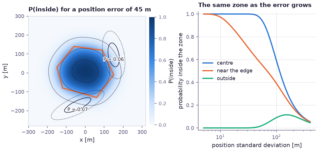
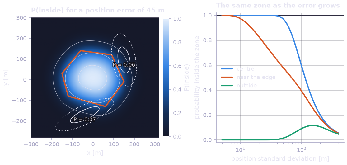
Left: the probability that a position with a 45 m standard error lies in the zone (orange outline), for every intended position on the map, and two anisotropic errors drawn as their one and two sigma ellipses. Right: how the probability changes as the error grows, for an aim point in the centre, near the edge and outside.

p_map = physics.gaussian_polygon_probability(aim_points, np.array([45.0, 0.0, 45.0]), zone)
# the Cholesky factor (l00, l10, l11) may carry a batch dimension, here one per sigma
p_sigma = physics.gaussian_polygon_probability(aim, np.stack([s, 0 * s, s], -1), zone)

Used for landing and drop zones, impact and debris footprints, GNSS position error against geofences, and the chance that an uncertain source lies in a protected area. Exact, with exact gradients with respect to the mean, the covariance and every vertex, so the aim point or the zone can be optimised.

Areas of intersections: overlap_area

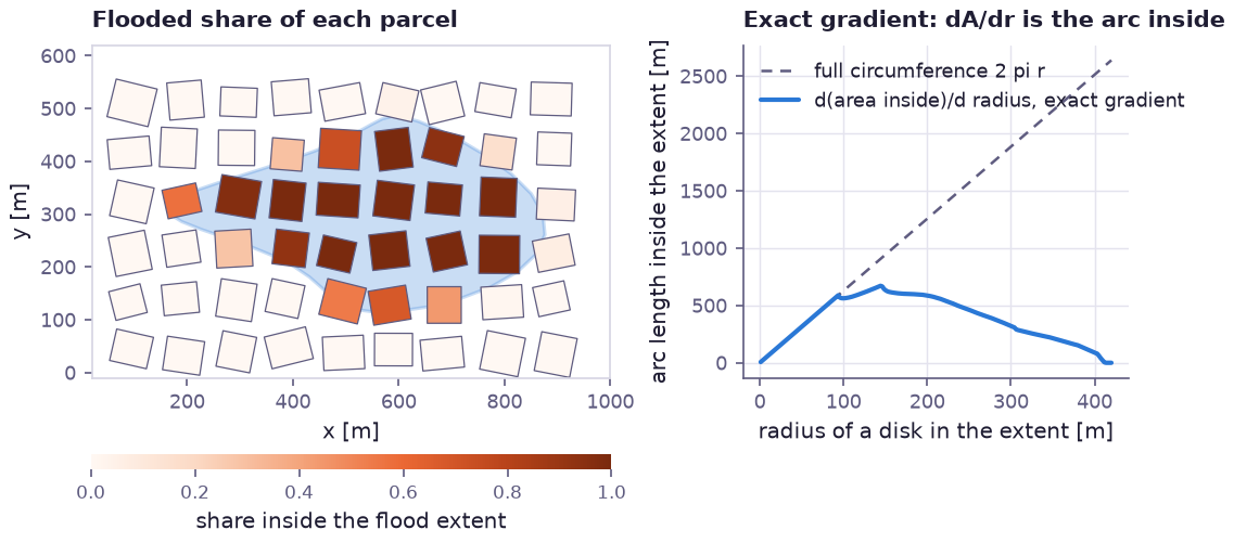
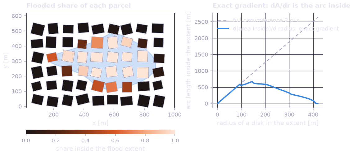
Left: the share of each of 54 parcels that lies inside a flood extent, in one batched call. Right: the derivative of the area of a disk inside the extent with respect to the radius, taken by automatic differentiation. It equals the length of the circle that lies inside the extent: the full circumference until the disk reaches the boundary, less afterwards.

share = physics.overlap_area(parcels, flood).evaluate() / parcel_areas   # parcels [54, 4, 2]
area_inside = lambda r: physics.overlap_area(flood, disk=jnp.stack([x0, y0, r])).evaluate().sum()
arc_inside = jax.grad(area_inside)(150.0)

Used for exposure of assets to hazard footprints, land-use shares, sensor and service coverage, and blast or exclusion radii against sites.

Line integrals through rasters: ray_integral

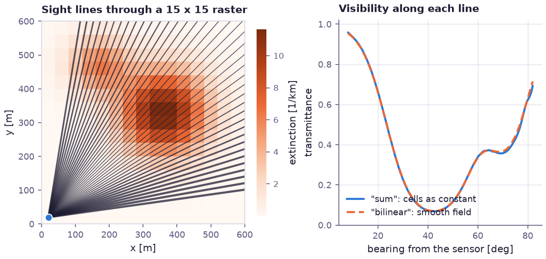
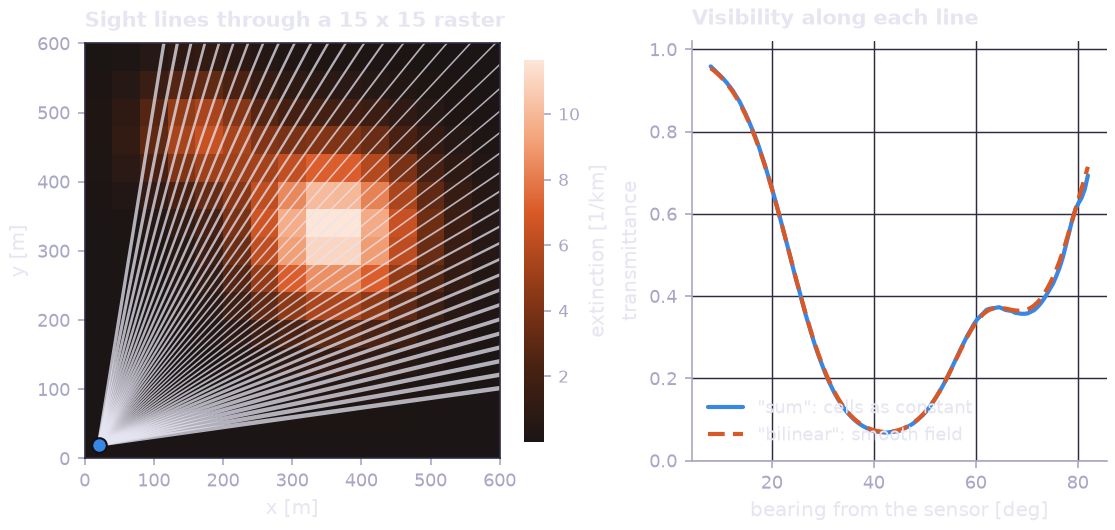
Left: 120 sight lines from a sensor through a 15 by 15 raster of smoke extinction (every third drawn, thicker where more light gets through). Right: the transmittance exp(-optical depth) along each line, with the raster read as constant cells and as a bilinear field.

depth = physics.ray_integral(extinction, segments, cell=(40.0, 40.0))            # [120]
depth_smooth = physics.ray_integral(extinction, segments, cell=(40.0, 40.0),
                                    reduce="bilinear", origin=(20.0, 20.0))
transmittance = prp.exp(-depth)

Used for optical depth and visibility, radio and line-of-sight obstruction (reduce="max"), travel cost along routes, and the length of a route inside a hazard (reduce="length_above").

Linear flow networks: network_potentials

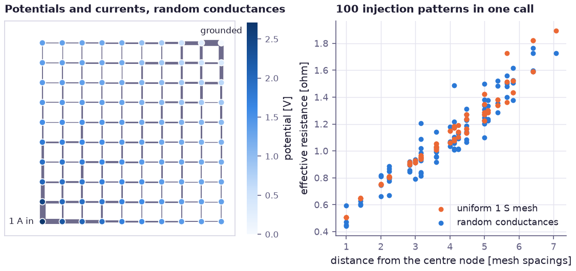
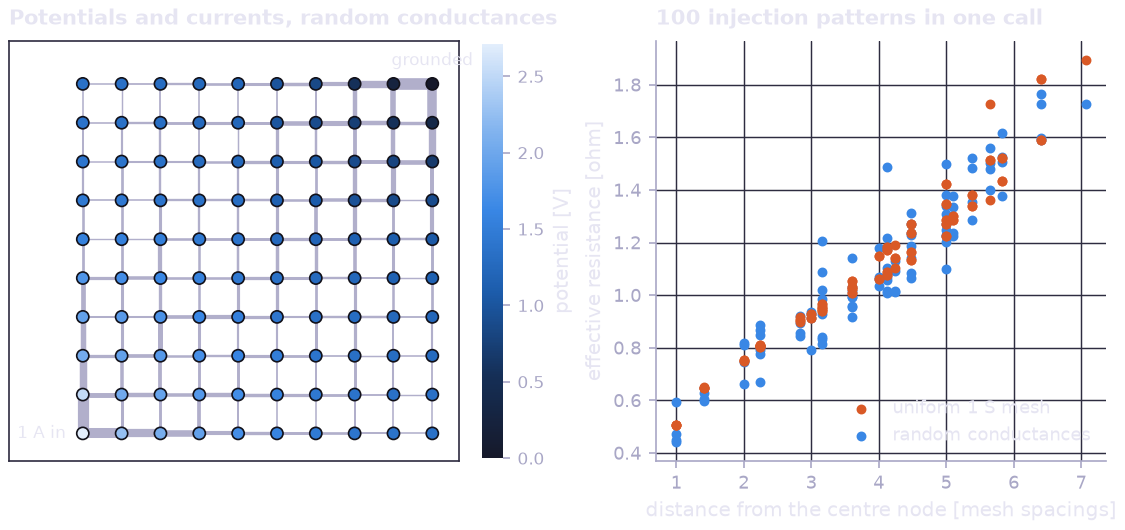
Left: a 10 by 10 mesh with random conductances, one ampere injected at a corner and drawn off at the grounded opposite corner; nodes are coloured by potential and lines are drawn thicker where more current flows. Right: the effective resistance between the centre and every other node, from one batched call with 100 injection patterns, for these conductances and for a uniform mesh.

phi = physics.network_potentials(edges, conductance, injection, ground=sink)
current = conductance * (phi[edges[:, 0]] - phi[edges[:, 1]])
# one solve per row of the injection matrix
phi_all = physics.network_potentials(edges, conductance, np.eye(n_nodes), ground=centre)

The same system is DC power flow (susceptances and bus angles, see Example: Transmission Grid Security and Cascading Outages), heat conduction between rooms or components, and linearised pipe and district heating networks.

Directional shadowing: directional_sweep

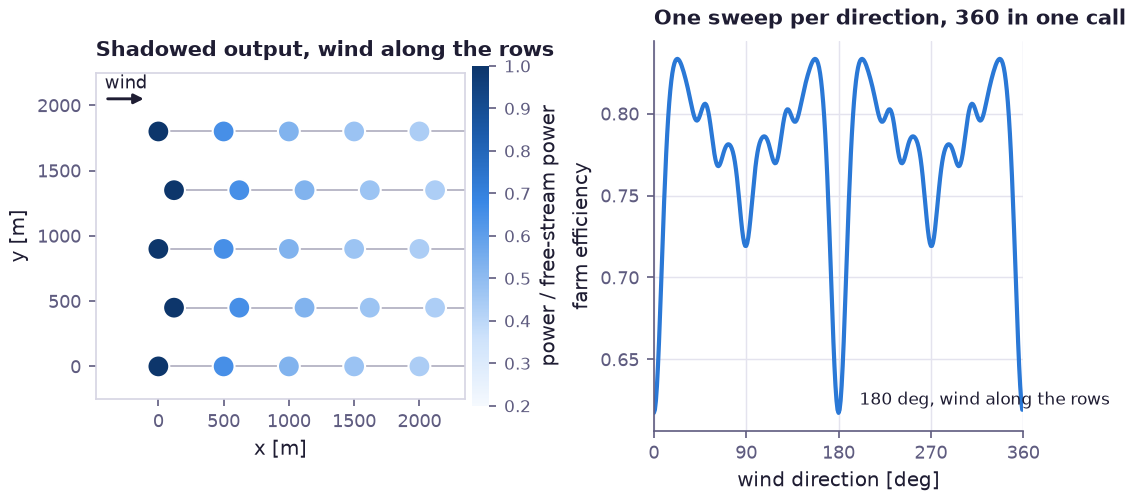
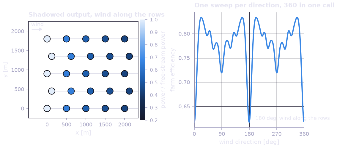
Left: the power of each turbine of a 25 turbine array, relative to an unshadowed turbine, with the wind blowing along the rows. Right: the efficiency of the whole array for every wind direction in one degree steps, evaluated in a single call with the direction as a batch dimension; the dips are the directions in which turbines line up.

speed = physics.directional_sweep(turbines, np.ones(25), direction=np.radians(np.arange(360.0)),
                                  strength=0.3, width=60.0, growth=0.06)   # [360, 25]
efficiency = (speed**3).mean(-1)

Used for wake losses in wind and tidal farms, shelter by trees and buildings, and any cascade in which upstream nodes reduce what reaches the nodes downstream.

Linear dynamics: propagate_linear

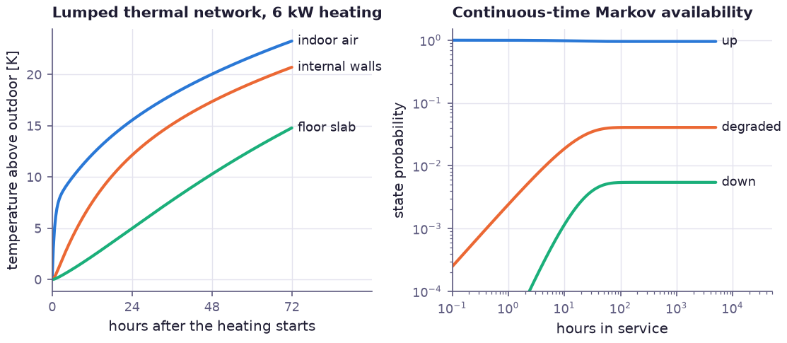
Left: a building as three heat capacities (air, internal walls, floor slab) coupled by conductances, heated with 6 kW from outdoor temperature. Right: a component that degrades, fails and is repaired, as a continuous-time Markov chain started in the up state. Each curve is one call with a vector of times.

temps = physics.propagate_linear(A, hours * 3600.0, np.zeros(3), heater)   # dT/dt = A T + u
probs = physics.propagate_linear(R, times, np.array([1.0, 0.0, 0.0]))       # dp/dt = R p

Used for compartment and box models (pharmacokinetics, pollutant fate), decay chains, lumped thermal and electrical circuits, and reliability and availability models.

Noisy time series: state_space_loglik

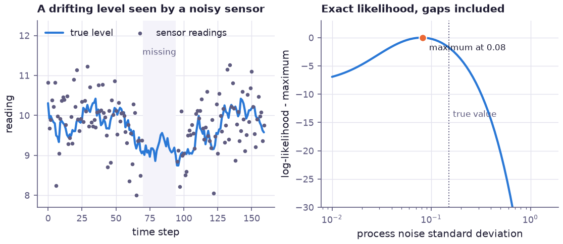
Left: a slowly drifting level read by a noisy sensor that drops out for 25 steps. Right: the exact log-likelihood of the readings as a function of the process noise, the gap handled by the filter itself.

ll = physics.state_space_loglik(readings[:, None], transition=np.eye(1), observation=np.eye(1),
                                process_cov=q**2 * np.eye(1), observation_cov=0.6**2 * np.eye(1),
                                initial_mean=np.array([10.0]), initial_cov=4.0 * np.eye(1))

Used to calibrate process models against sensor series with missing values: degradation and drift, water levels, temperatures and positions.

Published correlations: piecewise_polynomial

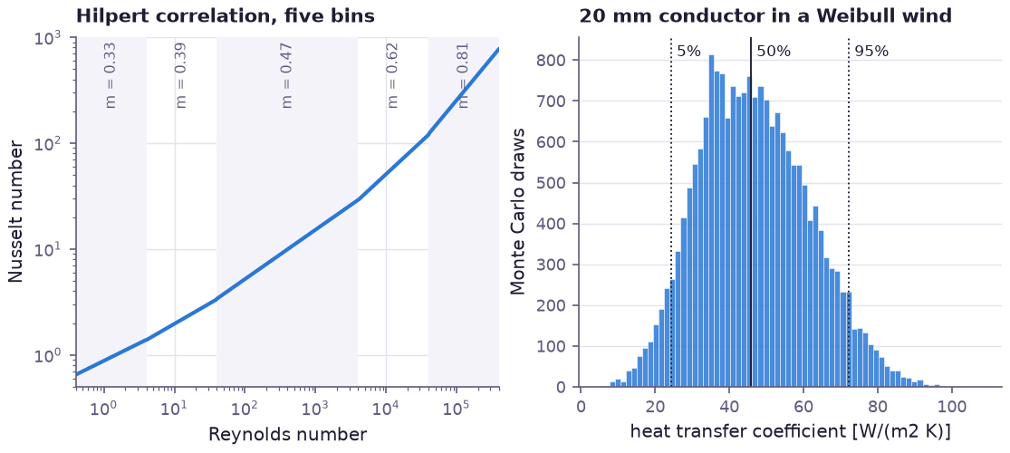
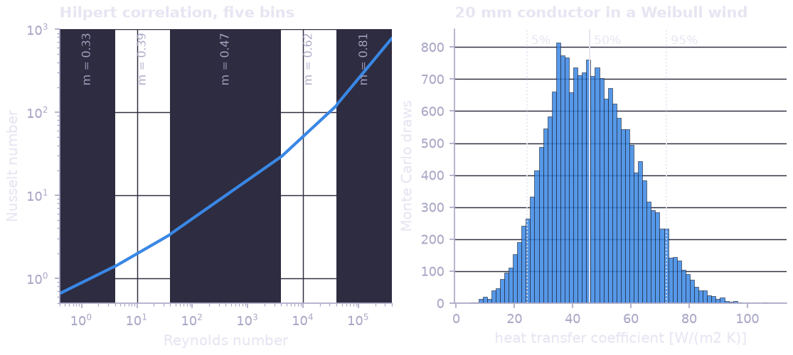
Left: the Hilpert correlation for a cylinder in cross flow, Nu = C Re^m Pr^(1/3) with five Reynolds number ranges, entered as its coefficient table. Right: the convective heat transfer coefficient of a 20 mm conductor in a Weibull distributed wind, drawn from the compiled model, with its 5, 50 and 95 percent quantiles.

coeffs = np.stack([np.log(C) + np.log(0.71) / 3, m], -1)          # ln Nu = ln C' + m ln Re
nusselt = physics.piecewise_polynomial(reynolds, breaks, coeffs, input="ln", output="exp")
wind = prp.RandomVariable("wind", prp.Weibull(scale=5.0, concentration=2.0))
h = physics.piecewise_polynomial(wind * 0.02 / 1.5e-5, breaks, coeffs,
                                 input="ln", output="exp") * 0.026 / 0.02

Used for heat and mass transfer correlations, blast and attenuation curves versus scaled distance, and any published fit given as a coefficient table.

Aggregate losses: compound_distribution

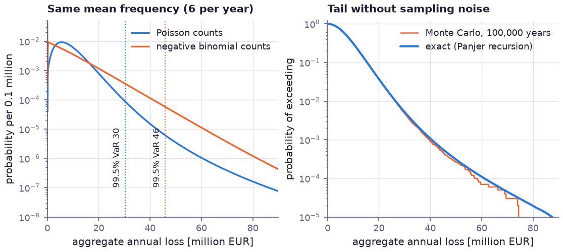
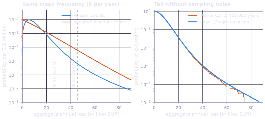
Left: the distribution of the annual aggregate loss with six losses a year on average and log-normal severities, for Poisson and for overdispersed negative binomial counts; the dotted lines mark the 99.5 percent value-at-risk. Right: the exact exceedance probability against 100 000 simulated years of the same model.

pmf = physics.compound_distribution(severity_pmf, rate=6.0, n_out=1200)
pmf_nb = physics.compound_distribution(severity_pmf, family="negative_binomial",
                                       shape=1.5, probability=4.0, n_out=1200)

Used for insurance and operational risk, outage and failure counts with random consequences, and any sum of a random number of random amounts. See Example: Aggregate Losses and a Stop-Loss Layer for reinsurance pricing on top of it.

Random fields: spectral_random_field

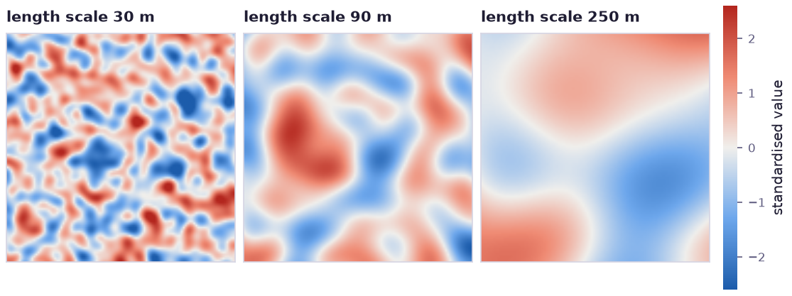
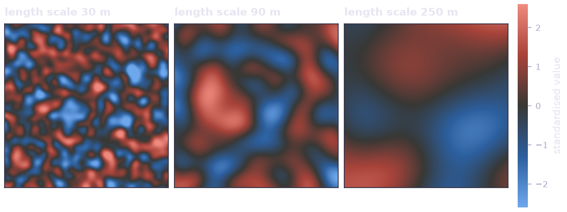
The same 400 spectral draws evaluated with three length scales of a squared exponential covariance. Because the draws are inputs, each realisation is a smooth function of the locations and of the length scale, which can therefore be calibrated.

modes = rng.normal(size=(400, 2))                 # spectral density of the covariance
phases = rng.uniform(0.0, 2 * np.pi, 400)
field = physics.spectral_random_field(points, modes, phases, length_scale=90.0, std=1.0)

Used for spatially correlated soil properties, rainfall and wind fields, material imperfections and terrain roughness.

Fatigue: fatigue_damage

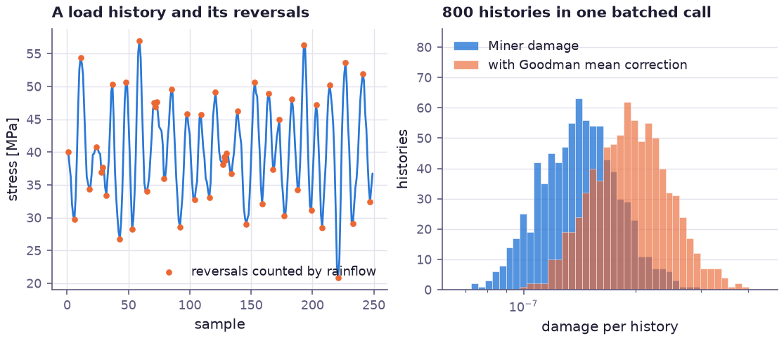
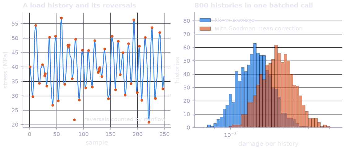
Left: a random stress history and the reversals that rainflow counting pairs into cycles. Right: the Palmgren–Miner damage of 800 such histories for an S–N curve with exponent 3, with and without the Goodman correction for the 40 MPa mean stress.

damage = physics.fatigue_damage(histories, sn_exponent=3.0, sn_coefficient=2.0e12)   # [800]
damage_goodman = physics.fatigue_damage(histories, sn_exponent=3.0, sn_coefficient=2.0e12,
                                        ultimate_strength=400.0)

Used for welded details, bridges and rails, wind turbine and offshore structures, and any component whose life is set by cycles of load. See Example: Fatigue of a Railway Bridge Detail.

Special functions

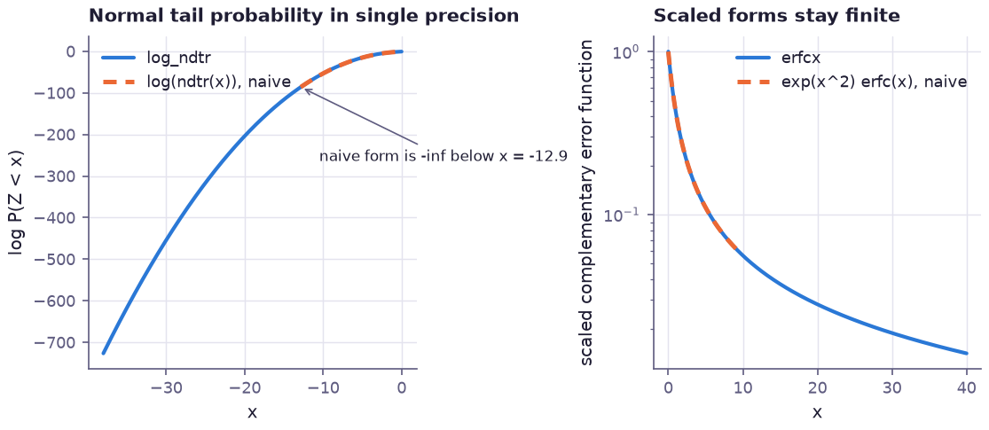
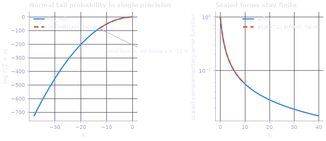
In single precision the logarithm of the normal lower tail computed as log(ndtr(x)) becomes minus infinity below x = -12.9, and exp(x^2) erfc(x) overflows beyond x = 9. The tail-accurate forms stay exact across the whole range, which keeps likelihoods of rare events and closed-form solutions finite.

from prophys.symbolic import erfcx, log_ndtr

log_ndtr(x)     # log P(Z < x), exact far into the tail
erfcx(x)        # exp(x**2) * erfc(x), no overflow

Composing a model

A Gaussian plume concentration is the steady kernel scaled by the emission rate over the wind speed; the wind direction and speed may be random variables:

import numpy as np
import prophys as prp
from prophys import physics

receptors = np.array([[250.0, 10.0, 1.5], [400.0, -30.0, 1.5]])
source = np.array([[0.0, 0.0, 20.0]])
concentration = physics.superpose(
    receptors,
    source,
    [emission_rate / wind_speed],
    direction=wind_direction,
    spread_across=(0.22, 0.9),
    spread_vertical=(0.2, 0.85),
    vertical="reflect",
    lid=800.0,
    images=3,
)

The Theis drawdown around a pumping well uses the radial kernel with radial_scale = 4 T t / S:

drawdown = physics.superpose(
    wells, pump, [q / (4 * np.pi * transmissivity)],
    kind="radial_exp1", radial_scale=4 * transmissivity * t / storativity,
)

Choosing between a primitive and symbolic code

A formula that is a handful of elementary operations per element (an Arrhenius rate, a friction factor from an explicit correlation, a probit) belongs in symbolic code. The primitives exist where a native kernel adds something the symbolic layer cannot: loops over pairs, samples and time steps, special functions and tail-accurate forms, discrete structure (traversals, recursions, cycle counting), or the size gate.