Example: Transmission Grid Security and Cascading Outages

A transmission planner has to know how power redistributes when injections change or a line trips, how likely the grid is to overload under uncertain wind and demand, how far a cascade of overload trips spreads once it starts, and which reinforcements buy the most security per euro. This chapter answers all four questions for a 24-bus, 230 kV meshed grid with one model: the DC power flow is network_potentials(), the flow sensitivities (PTDF and LODF) come from its gradient, wind, demand and the initiating fault are random variables marginalised by Monte Carlo with standard errors, and the line uprates are optimised by gradient descent. The full runnable source is examples/power_flow/model.py.

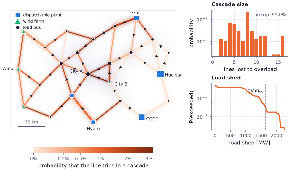
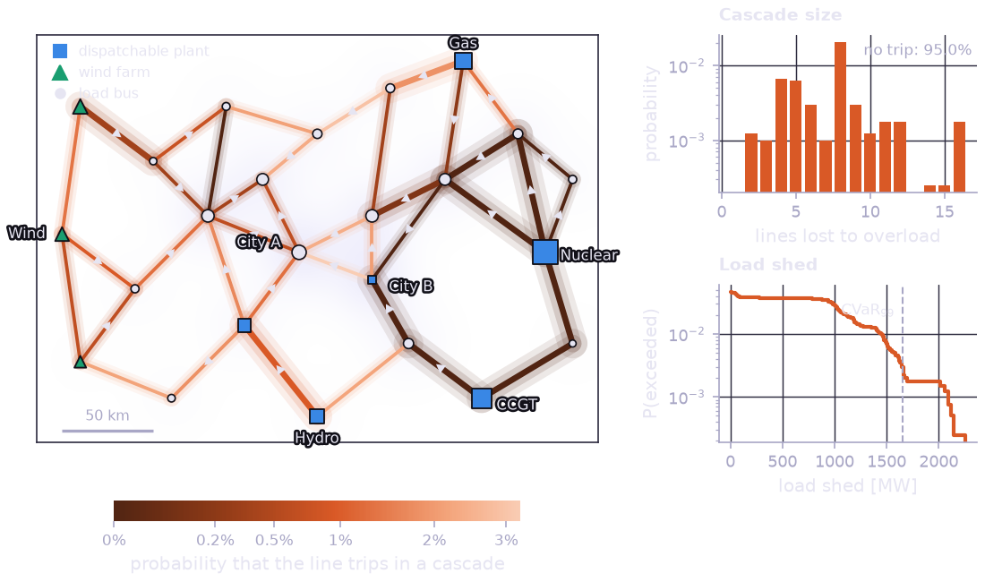
The grid in plan view. Each line is coloured by the probability that it trips on overload during a cascade started by a random single-line fault, under random wind and demand; double circuits are drawn thicker and the arrowheads show the direction of the mean flow. Squares are dispatchable plants, triangles wind farms and dots load buses, sized by their mean output or demand. The highest trip probabilities, 2 to 3 %, are on the lines into City B (5-21, 5-6, 6-21), on the route from the gas plant towards City A (14-15, 15-16, 15-22) and on the hydro connection 2-3. Right: 95 % of initiating faults stay isolated, but the cascades that do start are large (61 % of them lose eight or more lines), and the load shed has a heavy tail up to about 2 GW.

Step 1 — The network and the DC power flow

Buses have plan-view coordinates in a grid frame and the lines are a fixed (m, 2) connectivity array, so a Network gives the line lengths. The series reactance of a 230 kV circuit, 0.49 Ω/km, gives each line’s DC susceptance b = V² / X in MW per radian:

grid = prp.Network(BUS_XY, LINES, site)
LENGTH_KM = np.asarray(grid.edge_lengths().evaluate())  # [km]

# DC power flow susceptance of a line: b = V^2 / X [MW/rad], with a series
# reactance of 0.49 ohm/km per 230 kV circuit (parallel circuits add).
V_KV = 230.0
X_OHM_PER_KM = 0.49
B_MW_PER_RAD = CIRCUITS * V_KV**2 / (X_OHM_PER_KM * LENGTH_KM)

The DC power flow B θ = P is a grounded Laplacian system, which is exactly what network_potentials() solves, with the reference bus as ground. Line flows are b (θ_i − θ_j):

theta = physics.network_potentials(LINES, B_MW_PER_RAD, injection, ground=SLACK)  # [rad]
flow = (theta[..., FROM] - theta[..., TO]) * B_MW_PER_RAD  # (..., n_line) [MW]
loading = prp.abs_(flow) / RATING_MW  # fraction of the thermal rating

injection is itself an expression of the uncertain inputs (step 3), so flow evaluates for one operating state or for a whole Monte Carlo batch of states in a single call.

Step 2 — PTDF from the gradient, LODF from the PTDF

The power transfer distribution factor PTDF[l, i] is the change of the flow on line l per MW injected at bus i and withdrawn at the reference bus. It is the Jacobian of the flow with respect to the injections; the DC flow is linear, so the Jacobian at any point is exact. The line outage distribution factor follows from it with the standard formula LODF[l, k] = PTDF_lk / (1 − PTDF_kk), where PTDF_lk is the flow on l per MW transferred between the two ends of line k:

def ptdf_matrix(susceptance=B_MW_PER_RAD):
    """PTDF[l, i] = d flow_l / d injection_i (withdrawn at the slack bus).
    The DC flow is linear, so the Jacobian at any point is exact."""
    return jax.jacrev(lambda p: dc_flows(susceptance, p))(jnp.zeros(N_BUS))


def lodf_matrix(ptdf):
    ...
    ptdf_k = ptdf[:, FROM] - ptdf[:, TO]  # (n_line, n_line)
    lodf = ptdf_k / (1.0 - jnp.diag(ptdf_k))[None, :]
    return lodf.at[jnp.arange(N_LINE), jnp.arange(N_LINE)].set(-1.0)

The check re-solves the grid with each line removed. A batch of 39 susceptance vectors, row k with line k open, goes through one batched solve:

f0 = dc_flows(B_MW_PER_RAD, p)
susceptance_n1 = B_MW_PER_RAD * (1.0 - jnp.eye(N_LINE))  # row k: line k open
resolved = dc_flows(susceptance_n1, p)  # (n_line outages, n_line)
predicted = f0[None, :] + lodf.T * f0[:, None]

The LODF prediction and the re-solved flows agree to 3·10⁻¹² MW over all 39 outages.

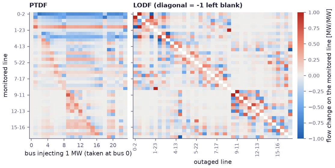
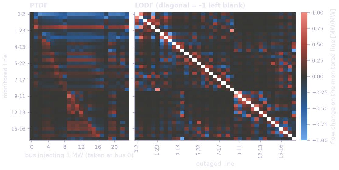
The two sensitivity matrices (every fifth line labelled). The PTDF columns show how an injection at each bus spreads over the grid on its way to the reference bus. The block structure of the LODF shows which lines back each other up. An outage in the western half of the grid (lines 9-10 to 19-20, lower right) moves its flow mostly onto other western lines. An outage in the eastern half moves it mostly onto other eastern lines.

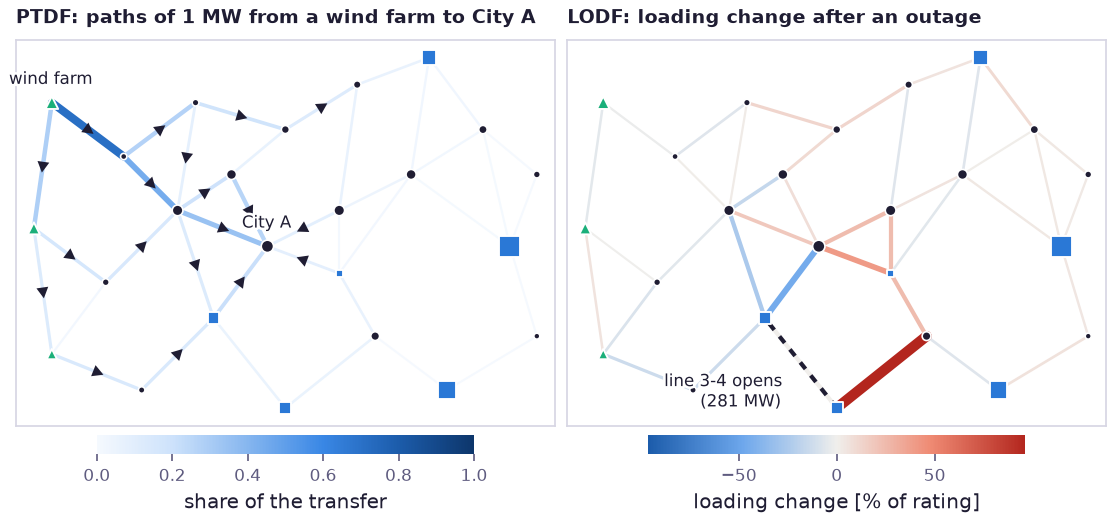
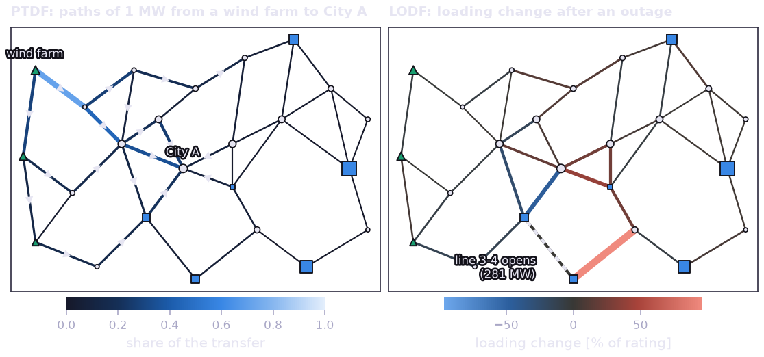
The same factors on the map. Left: a PTDF difference, the paths taken by 1 MW moved from the northern wind farm to City A; line width and colour give the share of the transfer, arrows its direction. Right: an LODF column in the nominal state. When line 3-4 opens, its 281 MW move almost entirely onto line 2-3 out of the hydro plant, and the central lines are partly relieved.

Step 3 — Uncertain wind, demand and faults

The hub-height wind speed is Weibull, shared by the three western wind farms through a generic cubic power curve. System demand has a common level (Gaussian, 7 %) and independent bus-level noise (4 %). A forced outage strikes a line with probability proportional to its length. The dispatchable plants share the residual demand in proportion to their capacity:

wind_speed = prp.RandomVariable("wind_speed", prp.Weibull(scale=8.5, concentration=2.0))  # hub height [m/s]
load_level = prp.RandomVariable("load_level", prp.Gaussian(1.0, 0.07))  # system demand / nominal
load_noise = prp.RandomVariable("load_noise", prp.Gaussian(jnp.zeros(N_BUS), 0.04 * jnp.ones(N_BUS)))
# A forced outage strikes a line with probability proportional to its length.
OUTAGE_PROB = LENGTH_KM / LENGTH_KM.sum()
initiating_line = prp.RandomVariable("initiating_line", prp.Categorical(jnp.asarray(OUTAGE_PROB)))

demand = load_level[..., None] * (1.0 + load_noise) * LOAD_MW  # (..., n_bus) [MW]
wind_mw = wind_capacity_factor(wind_speed)[..., None] * WIND_CAP_MW  # (..., n_bus) [MW]

residual = prp.sum_(demand, axis=-1) - MUST_RUN_MW.sum() - prp.sum_(wind_mw, axis=-1)
dispatch_frac = prp.clip(residual / DISPATCH_CAP_MW.sum(), 0.0, 1.0)
injection = dispatch_frac[..., None] * DISPATCH_CAP_MW + wind_mw + MUST_RUN_MW - demand  # (..., n_bus)

Evaluating flow with 4000 draws of these inputs gives the loading distribution of every line. Adding LODF[:, k] · flow_k gives the post-contingency flows for every single-line outage in every draw (N-1 screening), with no further solves.

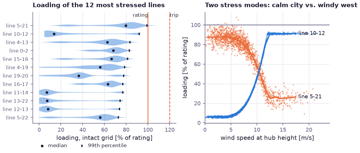
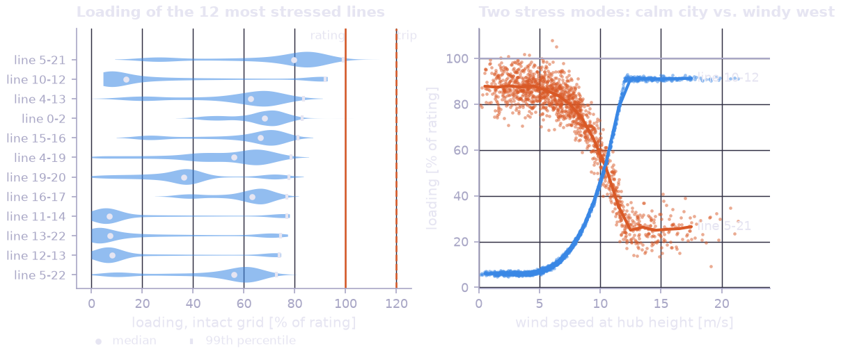
Left: intact-grid loading of the 12 lines with the highest 99th percentile. Line 5-21 into City B is the only one that regularly reaches its rating. Right: the grid has two stress modes. On calm days the thermal plants carry the load and line 5-21 runs close to its limit; on windy days it is unloaded, but the wind corridor 10-12 fills up to 91 % once the turbines reach rated power.

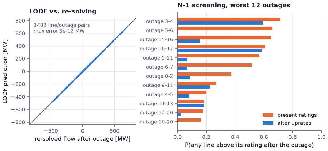
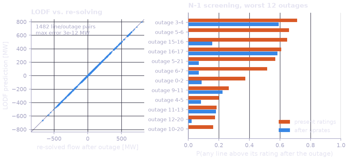
Left: the LODF check. Each dot is one line after one outage, re-solved flow against LODF prediction; all 1482 pairs lie on the diagonal. Right: N-1 screening, the probability over the uncertain states that some line exceeds its rating after each outage, for the 12 worst outages, with the present ratings and after the uprates of step 5. The outages of lines 3-4 and 16-17 stay insecure because they overload the remaining connection of a plant (2-3 for the hydro plant, 7-17 for the gas plant), and at this risk price the optimiser left both connections unreinforced.

Step 4 — Cascading outages

A cascade starts with the random initiating fault. It then runs for a fixed number of rounds (six). In each round the grid is split into its connected islands, and every island is re-dispatched on its own: its plants cover the island’s demand up to their capacity, surplus generation is curtailed and any deficit is shed pro rata. The DC flow is then solved again, and protection trips every line above its short-term emergency rating (1.2 times the continuous rating):

alive = 1.0 - jax.nn.one_hot(first_out, N_LINE)
lost_per_round = []
for _ in range(n_rounds):
    p, _ = balance_islands(island_labels(alive), demand_mw, wind)
    f = dc_flows(B_MW_PER_RAD * (alive + 1e-9 * (1.0 - alive)), p)
    trip = alive * (jnp.abs(f) > TRIP_FACTOR * rating)
    alive = alive - trip
    lost_per_round.append(trip.sum(axis=-1))
_, shed_bus = balance_islands(island_labels(alive), demand_mw, wind)
return jnp.stack(lost_per_round, axis=-1), alive, shed_bus.sum(axis=-1)

An open line keeps a susceptance of 10⁻⁹ times its own value, so the Laplacian stays positive definite when the grid splits. Each island is balanced before the solve, so no power crosses these ties. All 4000 cascades run together as one batch. The load shed is summarised with Monte Carlo standard errors by mean_error() and cvar_error().

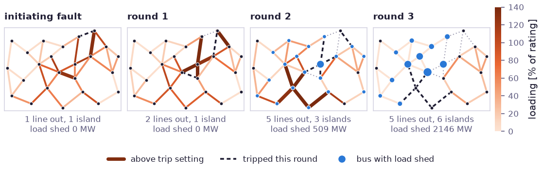
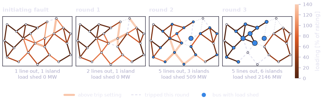
One cascade from the sample, round by round, with lines coloured by loading. A fault on line 16-17 out of the gas plant pushes line 7-17 and line 5-21 into City B past their trip settings. Their loss overloads the lines around bus 6 in the centre (round 2). That in turn overloads the southern lines around the hydro plant and bus 4 (round 3). The grid ends up as six islands and 2.1 GW of load is shed (blue buses, sized by the shed load).

Step 5 — Uprating lines by gradient descent

Reconductoring with high-temperature conductor raises a line’s rating without changing its reactance, so the flows stay the same and only the limits move. The uprates are a softplus-positive Param vector. The objective prices the expected number of overloaded lines, intact and after a random single outage and smoothed by a sigmoid so that it has a gradient, against the uprating cost:

uprate = prp.Param("uprate_mw", shape=(N_LINE,), init=10.0 * jnp.ones(N_LINE), transform="softplus")

def expected_overloads(rating, lodf):
    over = lambda f: prp.sigmoid((prp.abs_(f) / rating - 1.0) / SMOOTH)  # noqa: E731
    post = flow[..., None, :] + flow[..., :, None] * jnp.asarray(lodf).T  # (..., outage k, line l)
    n1 = prp.sum_(over(post) * (1.0 - jnp.eye(N_LINE)), axis=-1)  # (..., k)
    per_state = prp.sum_(over(flow), axis=-1) + prp.sum_(n1 * OUTAGE_PROB, axis=-1)
    return prp.mean(per_state)

cost = prp.sum_(uprate * (UPRATE_COST * LENGTH_KM))
objective = expected_overloads(uprate + RATING_MW, lodf) * RISK_PRICE + cost
result = prp.optimize(objective, wrt=[uprate], n_steps=200, learning_rate=2.0, extra_env=design_env)

design_env binds the random inputs to 400 Monte Carlo draws, so every gradient step sees the whole distribution of operating states and all 39 contingencies of each.

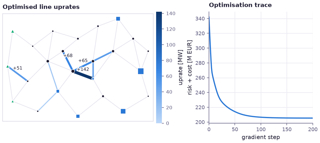
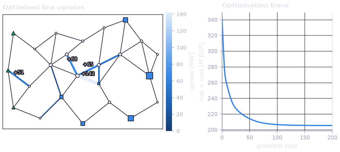
Left: the optimised uprates. The money goes to the short lines around City A and City B and to the wind corridor 10-12. Right: the objective (expected overload cost plus uprating cost) converges in about 100 gradient steps.

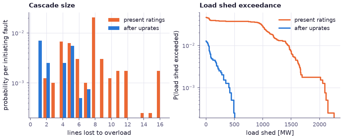
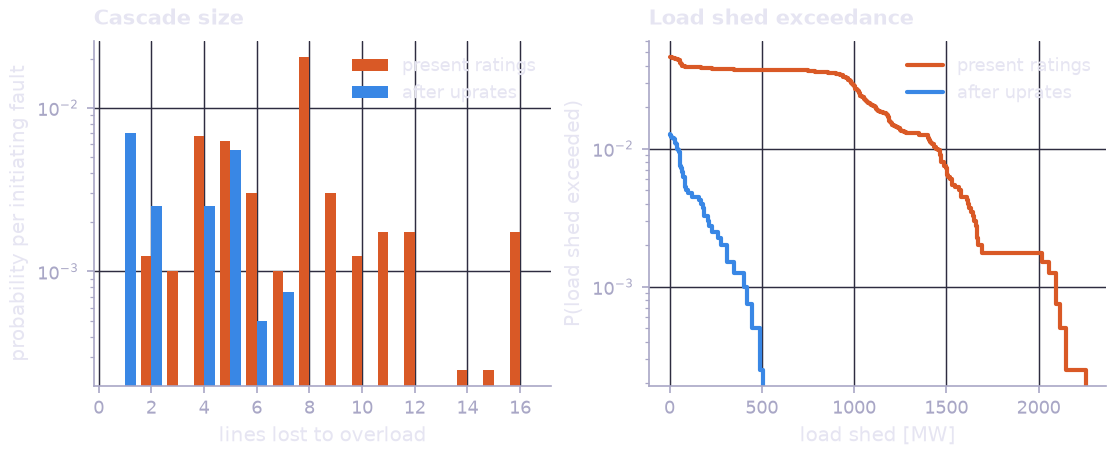
The same 4000 initiating faults and operating states, cascaded with the present and the uprated ratings. The 79 M EUR of uprates cut the probability of an overload trip from 5.0 % to 1.9 %. They remove the cascades that lose eight or more lines, and they bring the 1 % conditional tail of load shed (CVaR₉₉) down from 1650 MW to 172 MW.

Results

=== Network ===
buses 24, lines 39, total length 2055 km
LODF check: max |LODF prediction - re-solved flow| = 3.41e-12 MW over 39 outages

=== Security screening (Monte Carlo) ===
P(any overload, intact grid)         = 0.006
P(any overload | random N-1 outage)  = 0.156
  outage  3-4 : P(post-contingency overload) = 0.712
  outage  5-6 : P(post-contingency overload) = 0.659
  outage 15-16: P(post-contingency overload) = 0.647

=== Cascades (initiating fault + up to 6 rounds of overload trips) ===
P(at least one overload trip) = 0.050
EstimateWithError:
  expected load shed [MW] = 46.7912 +/- 3.766
  95% interval = [39.4102, 54.1722]
  relative error = 8.048%
  n_samples = 4000, ess = 4000.0 (iact 1.00)
TailRiskEstimate:
  VaR at 0.99 = 1443.66
  CVaR at 0.99 = 1649.87 +/- 48.21
  95% interval = [1555.37, 1744.37]
  tail draws = 40 of 4000

=== Design: line uprates ===
objective 330.3 -> 208.8 M EUR (expected overloads 0.330 -> 0.127, uprating cost 78.7 M EUR)
  line  5-21: 350 MW + 142 MW
  line  5-22: 250 MW + 68 MW
  line  5-6 : 350 MW + 65 MW
  line 10-12: 250 MW + 51 MW
  line  6-7 : 700 MW + 49 MW
  line  6-21: 250 MW + 43 MW
P(overload trip) 0.050 -> 0.019; E[load shed] 46.8 -> 1.8 MW; CVaR99[load shed] 1650 -> 172 MW

Running it

$ python examples/power_flow/model.py

The run takes about ten seconds on a laptop CPU.