Example: Population Pharmacokinetics and Dose Design

A new oral drug is given twice daily. It works when the plasma concentration stays above 4 mg/L and causes dose-limiting toxicity above 20 mg/L, and the same dose produces very different concentrations in different patients. This example learns the population kinetics from sparse, noisy monitoring samples, some of them below the assay’s limit of quantification, and then designs a loading and maintenance dose that maximises the expected time inside the therapeutic window with at most a 10 % probability of a toxic peak. The compartment model is solved exactly by the matrix exponential of propagate_linear(), between-patient variability enters as log-normal random variables, censored samples go into the fit as Observations, and the regimen is optimised by gradient descent with optimize(). The full runnable source is examples/pharmacokinetics/model.py.

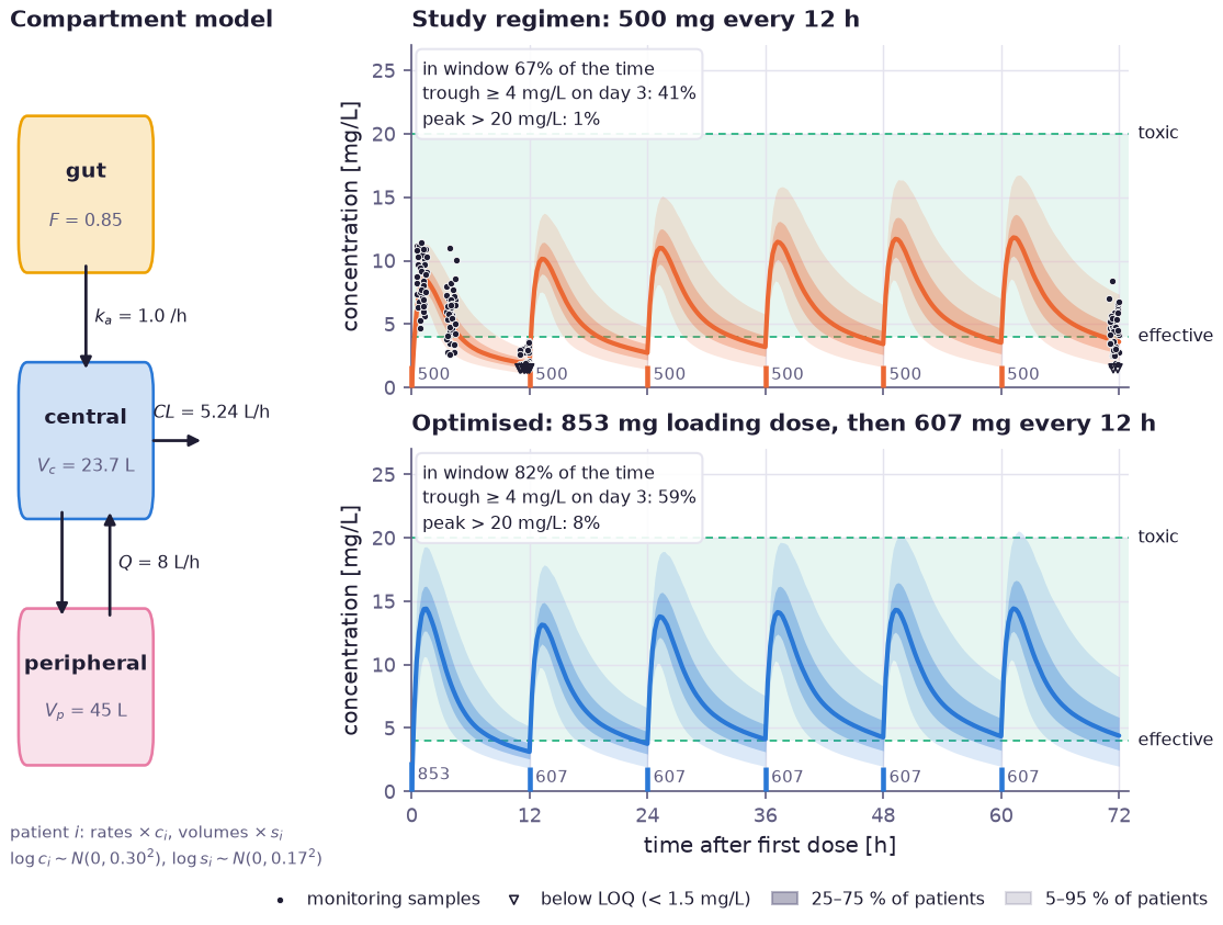
Plasma concentration over the first three days in 2 000 virtual patients drawn from the calibrated population: the median (line), the middle half (dark band) and 90 % of patients (light band), with the therapeutic window shaded between 4 and 20 mg/L and the doses marked on the time axis. Top: the study regimen, with the 160 monitoring samples it produced (triangles are results below the 1.5 mg/L quantification limit). Its troughs fall below the window in most patients. Bottom: the optimised regimen. A loading dose brings patients into the window on the first day and a larger maintenance dose lifts the troughs, while the peaks stay below the toxic threshold in more than 90 % of patients.

Step 1 — The compartment model

Drug amounts in the gut, the central (plasma) compartment and a peripheral tissue compartment obey a linear system \(dA/dt = K A\): first-order absorption with rate \(k_a\), elimination with clearance \(CL\) from the central volume \(V_c\), and exchange with the peripheral volume \(V_p\) at the intercompartmental clearance \(Q\). The typical clearance and central volume are parameters to be learned. The generator is an ordinary symbolic matrix of them:

clearance = prp.Param("CL", init=3.5, transform="softplus")  # typical clearance [L/h]
v_central = prp.Param("Vc", init=35.0, transform="softplus")  # typical central volume [L]

generator = prp.stack(
    [
        prp.stack([-KA, 0.0, 0.0]),
        prp.stack([KA, -(clearance + Q_INTER) / v_central, Q_INTER / V_PERIPHERAL]),
        prp.stack([0.0, Q_INTER / v_central, -Q_INTER / V_PERIPHERAL]),
    ]
)  # [1/h], (3, 3)
UNIT_DOSE_IN_GUT = jnp.array([1.0, 0.0, 0.0])


def central_fraction(duration) -> prp.Expr:
    return physics.propagate_linear(generator, duration, UNIT_DOSE_IN_GUT)[..., 1]

propagate_linear() returns \(e^{K t} A_0\) without discretising time: there is no step size to tune and no integration error, and the gradient with respect to the generator (and so to \(CL\) and \(V_c\)) and to the duration is exact.

Step 2 — Patients as random variables

Each patient gets a rate factor \(c_i\) that scales every first-order rate constant and a size factor \(s_i\) that scales every volume, both log-normal with median one. A patient’s clearance is then \(CL\,c_i s_i\) and their curve is the typical curve on a stretched time axis (Dedrick’s pharmacokinetic time), so one generator serves the whole population. Repeated doses add up by superposition because the system is linear:

clock = prp.RandomVariable("clock", prp.LogNormal(0.0, omega_clock))
size = prp.RandomVariable("size", prp.LogNormal(0.0, omega_size))


def concentration(t: float, doses, clock_factor=clock, size_factor=size) -> prp.Expr:
    total = 0.0
    for dose, t_dose in zip(doses, DOSE_TIMES):
        if t_dose < t:
            total = total + dose * central_fraction(clock_factor * (t - t_dose))
    return BIOAVAILABILITY * total / (v_central * size_factor)

The spreads omega_clock and omega_size are themselves parameters, learned along with \(CL\) and \(V_c\).

Step 3 — Sparse monitoring and censored samples

In the monitoring study each of 160 patients on 500 mg every 12 h gave one blood sample, at 1, 4, 11.5 or 71.5 h after the first dose. A measured concentration is log-normal around the patient’s true concentration with the assay’s 12 % error. Each sampling time is one attribute, and the compiled model marginalises the patient factors by Monte Carlo:

measured = {
    t: prp.UncertainAttribute(
        f"conc_{t:g}h",
        prp.LogNormal(mu=prp.log(concentration(t, [STUDY_DOSE] * 6)), sigma=ASSAY_CV),
        unit="mg/L",
        domain=f"measured plasma concentration {t:g} h after the first 500 mg dose",
    )
    for t in SAMPLING_TIMES
}
model = prp.ProbabilityModel(*measured.values())

Eighteen of the samples, mostly troughs, came back as “< 1.5 mg/L”. Handing them to the fit as left-censored observations makes each one contribute \(\log P(C \le 1.5)\) instead of a made-up value. All four sampling times are fitted together with finetune():

observations = {f"conc_{t:g}h": prp.Observations.detection_limit(v, limit=LOQ) for t, v in record.items()}
fit = prp.finetune(compiled, observations, n_steps=400, learning_rate=0.1)

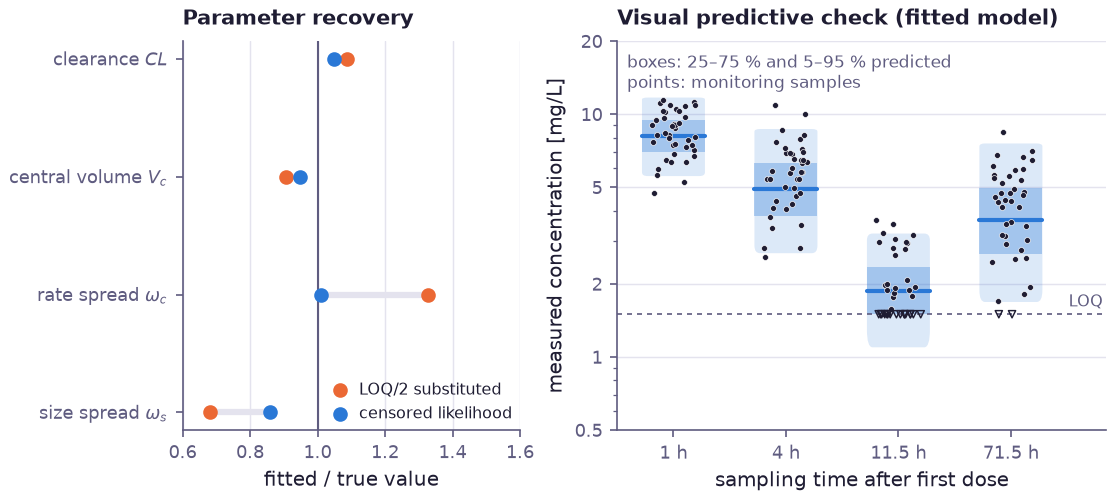
Left: fitted population parameters relative to the values that generated the record. The censored likelihood recovers all four parameters, including the between-patient spread of the rates. Substituting LOQ/2 for every non-detect puts fabricated low values into the troughs, inflates the rate spread by a third and shrinks the size spread. Right: visual predictive check. The boxes are the 25–75 % and 5–95 % ranges of the measured concentration predicted by the fitted model at each sampling time; the points are the monitoring samples, non-detects drawn as triangles at the quantification limit.

Step 4 — Target attainment, toxicity and the optimal regimen

With the fitted parameters, 2 000 virtual patients are drawn from the population distributions. Every regimen on the twice-daily schedule is a weighted sum of the unit-dose responses responses[..., k] (the concentration caused by 1 mg given at the k-th dosing time), so the matrix exponentials are evaluated once. The expected fraction of time inside the window, with the window edges relaxed by logistic functions, is maximised over the loading and maintenance doses subject to a probability of a toxic peak of at most 10 %:

loading = prp.Param("loading_dose_100mg", init=5.0)  # [100 mg]
maintenance = prp.Param("maintenance_dose_100mg", init=5.0)  # [100 mg]
resp = jnp.asarray(responses)
conc = 100.0 * (loading * resp[..., 0] + maintenance * prp.sum_(resp[..., 1:], axis=-1))
width = 0.4  # [mg/L] softness of the window edges
in_window = prp.sigmoid((conc - C_EFFECTIVE) / width) * prp.sigmoid((C_TOXIC - conc) / width)
expected_time_in_window = prp.mean(in_window)
peak = prp.softmax(conc, axis=-1, tau=0.25)  # per patient [mg/L]
toxicity = prp.mean(prp.sigmoid((peak - C_TOXIC) / width))
opt = prp.optimize(
    -expected_time_in_window,
    wrt=[loading, maintenance],
    constraints=[toxicity - TOXICITY_BUDGET],
    n_steps=300,
    learning_rate=0.05,
)

The probability of target attainment of the study regimen can also be read straight off the compiled model, as the Monte Carlo probability that the measured day-3 trough reaches 4 mg/L: 1 - compiled.prob("conc_71.5h", C_EFFECTIVE, params=fit.raw_params, n_samples=4000).

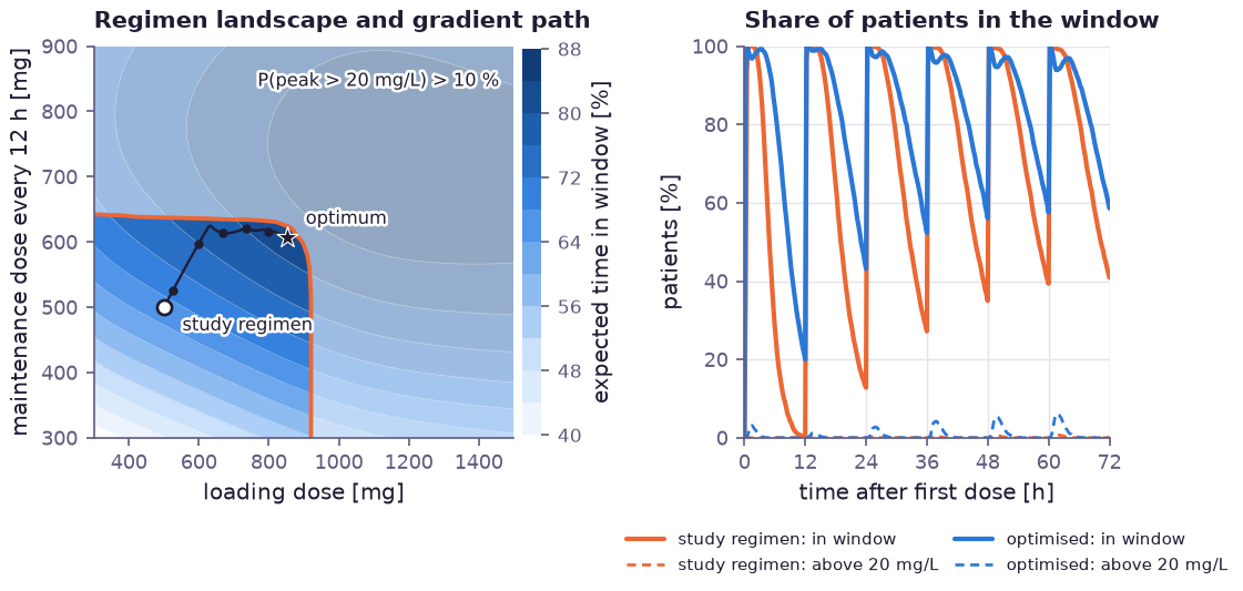
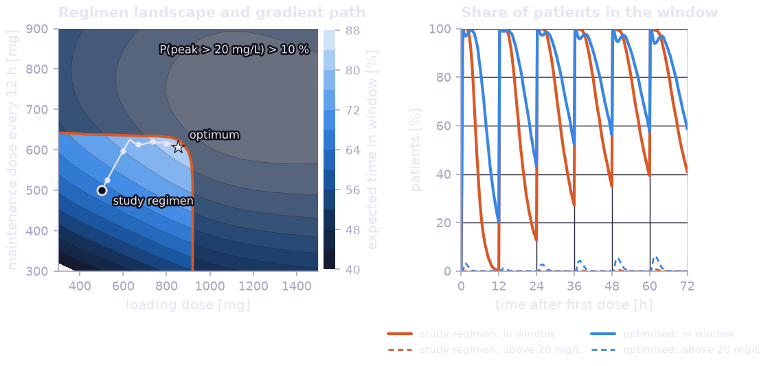
Left: expected time in the therapeutic window over the first three days for every combination of loading and maintenance dose, evaluated exactly on the virtual population. The veiled region is excluded by the toxicity constraint, whose boundary is the orange line. The gradient path starts at the study regimen, climbs the landscape and ends on the constraint boundary: larger doses would add time in the window but push more than 10 % of patients above 20 mg/L. Right: share of patients inside the window (solid) and above the toxic threshold (dashed) over time. The loading dose closes the first-day gap and the higher maintenance dose keeps most troughs above 4 mg/L.

Results

The console output of python examples/pharmacokinetics/model.py:

=== Population calibration (160 patients, 18 below LOQ) ===
  CL           fitted   5.242   true   5.000
  Vc           fitted  23.706   true  25.000
  omega_clock  fitted   0.303   true   0.300
  omega_size   fitted   0.172   true   0.200
  final negative log-likelihood 293.3
  LOQ/2 substitution instead: CL 5.442, Vc 22.658, omega_clock 0.399, omega_size 0.136

=== Study regimen 500 mg q12h ===
  P(day-3 trough >= 4 mg/L) = 43.6%
  time in window 66.5%, target attainment 40.9%, toxicity 0.8%

=== Optimised regimen ===
  loading dose 853 mg, then 607 mg every 12 h
  time in window 81.8%, target attainment 58.6%, toxicity 8.4%

The probability from the compiled model (43.6 %) refers to the measured trough, which includes the assay error; the virtual-population figure (40.9 %) refers to the true trough. Even the optimal regimen reaches the target in only 59 % of patients: with this much variability between patients, no single dose fits everyone, which is the case for therapeutic drug monitoring and individual dose adjustment.

Primitives exercised

Feature	Used for
propagate_linear()	Exact matrix-exponential solution of the three-compartment model
RandomVariable, LogNormal	Between-patient rate and size factors; the assay error
Observations	Samples below the limit of quantification as left-censored data
finetune()	Joint Monte Carlo maximum likelihood over four sampling times
prob, optimize()	Target attainment; regimen design under a toxicity constraint

Running it

$ python examples/pharmacokinetics/model.py

The run takes about a minute on a laptop CPU. The figures on this page are produced by docs/generate_example_pharmacokinetics.py.