

Probabilistic Training#
A surrogate that feeds a risk model has to get more than its mean right.
Quantiles, CVaR and exceedance probabilities live in the tails of its
predictive distribution, and fine tuning scores observations by their log
density. This page covers the tools for training that distribution: output
heads with proper tails, losses that are proper scoring rules, training on
whole distributions instead of single values, and operational surrogates
that stand in for a whole model’s Monte Carlo answer (prophys.amortize()).
Everything on this page runs on the free tier, except the prior fitted network, whose prefix attention needs a license.
Predictive distributions and their tails#
Four heads give a predictive distribution, available as a prophys
distribution from s.distribution(...):
Head |
Predictive distribution |
|---|---|
|
A |
|
A |
|
A Gaussian with a predicted mean and standard deviation. |
|
A mixture of |
For the quantile and histogram heads the CDF, log density, quantile
function, mean, variance, CVaR (dist.cvar(alpha), the mean above the
alpha quantile, as cvar()), the
CRPS (dist.crps(y)) and reparameterised samples are all closed form.
Tails. A quantile head learns a handful of quantiles, say 0.05 to 0.95. The probability beyond them has to go somewhere, and where it goes decides every risk number above the 95 percent level. prophys attaches a tail whose density at the outermost quantile equals the density of the adjacent segment, so the density has no jump, and whose shape is:
"exponential"(the default): unbounded support. With finely spaced outer levels (0.99, 0.995) it reproduces the CVaR of a Gaussian at 99 percent within one percent."halfnormal": unbounded, lighter than exponential."linear": the linear extension of the quantile function to the levels 0 and 1, the only behaviour before prophys 0.3. It bounds the support, so an observation beyond it had a log density of-1e30, which stalled fine tuning. It is kept for reproducing old results.
The histogram head uses the same rule. Its outer bins are replaced by tails
whose density continues that of the adjacent bin. Their length therefore
follows the learned probabilities, not the width of the outer bin, which is
set by the most extreme training target. With two bins or fewer, half of each
tail’s mass lies within one outer bin width instead (Muller et al. 2022).
tails="none" keeps the outer bins uniform and the support bounded.
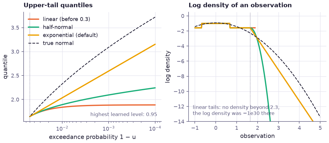
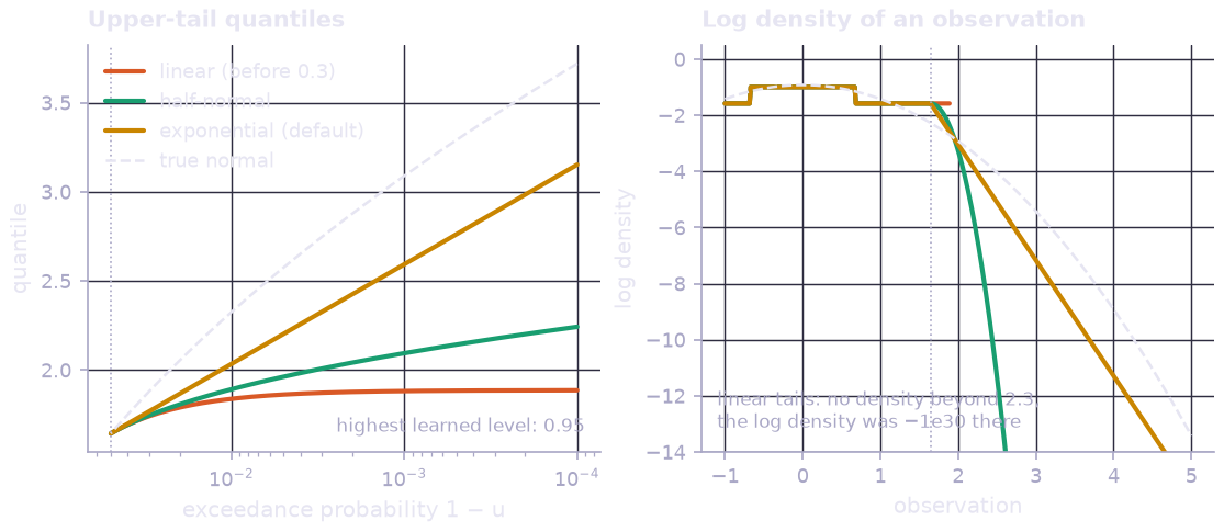
A quantile head with the levels 0.05, 0.25, 0.5, 0.75 and 0.95, set exactly to the quantiles of a standard normal. Left: upper-tail quantiles beyond the highest learned level. The linear extension flattens out at 1.9 and the half-normal tail is lighter still than the exponential one, which stays closest to the normal. Right: the log density; beyond 2.3 the linear tail has none at all. With only five levels the tail density is matched to a wide segment, so even the exponential tail is short: its CVaR at 99 percent is 2.28 against the true 2.67 (half-normal 1.98, linear 1.86). Learn levels near the quantiles you serve, or use a histogram head, which learns the tail probability itself.
Losses#
pretrain() takes a loss name, or a mapping from loss
names to weights for a weighted mix:
nn.pretrain(s, x, y, loss="hl_gauss")
nn.pretrain(s, x, y, loss={"hl_gauss": 1.0, "mse": 0.1})   # a weighted mix
Loss |
Head |
What it is |
|---|---|---|
|
histogram |
The default for a histogram head. Cross entropy against an HL-Gauss
target: a Gaussian around each observation integrated over the bins,
with a standard deviation of |
|
histogram |
Cross entropy against the hard histogram of the targets. With a fresh draw every step it is the KL divergence to the true distribution plus a constant (the prior fitted network loss, Muller et al. 2022). |
|
histogram |
The KL divergence from the target bin probabilities to the predicted ones. Same gradient as the cross entropy, but it is zero exactly at the target, so its value is readable. Meant for distribution targets. |
|
any probabilistic head |
The continuous ranked probability score in closed form: Gaussian (Gneiting et al. 2005), mixture (Grimit et al. 2006), quantile and histogram heads with their tails. It grows linearly with the error, so it is more robust to outliers than a likelihood. |
|
Gaussian |
The Gaussian likelihood weighted by the predicted variance to the
power |
|
quantile, Gaussian, mixture |
The natural losses of these heads, unchanged. |
|
any |
Point losses on the point prediction (for a histogram head its mean). Useful as a small term in a mix. |
Every probabilistic loss above is a proper scoring rule. Its expected value under the true distribution is lowest when the prediction is that distribution, so a lower loss means a better distribution, not only a better mean. The test suite checks this numerically for each loss.
Which one to use:
Deterministic simulator sweeps (a CFD grid, a wake model): keep a point head and
"mse". Distributional losses gain nothing when the target has no noise.Noisy targets (SCADA data, observed loads, single Monte Carlo draws): a histogram head with
"hl_gauss", or a Gaussian or mixture head with"crps". The histogram head makes no shape assumption; add{"mse": 0.1}when the point prediction matters most.Risk outputs: quantile or histogram heads with the default exponential tails, and check
card.tail_pinball(below).Distribution targets (next section): a histogram head with
"kl".
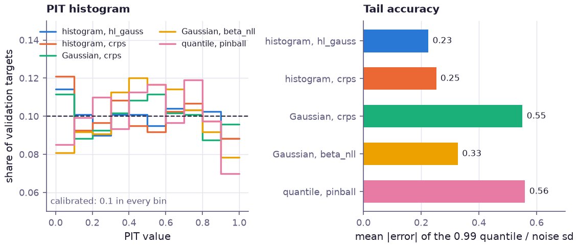
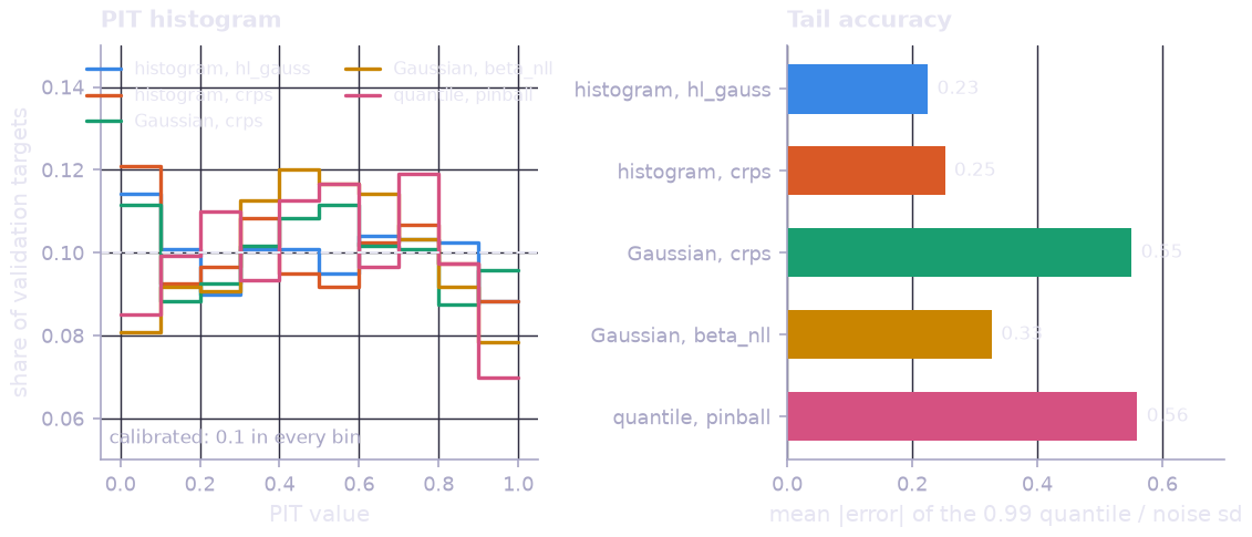
Five surrogates trained on the same 6000 noisy rows, with heteroscedastic Student-t noise (5 degrees of freedom). Left: the PIT histograms of the validation split are all within about 0.02 of the flat line of a calibrated distribution. Right: the mean error of the predicted 0.99 quantile against the truth, in units of the local noise standard deviation. The histogram heads learn the heavier tail (0.23 and 0.25). The Gaussian heads cannot represent it; the beta-weighted likelihood does better than CRPS here (0.33 against 0.55). The five-level quantile head, whose 0.99 quantile comes from its tail beyond the 0.95 level, is no better than the Gaussian (0.56).
Distribution targets#
A prophys model can say more about its outputs than one value per input.
It can give many Monte Carlo draws, or an exact CDF. Training on the whole
distribution instead of one draw lowers the variance of the loss by up to the
number of draws (Hinton et al. 2015; Menon et al. 2021). target_kind
tells pretrain() what the targets are:
|
|
Use |
|---|---|---|
|
|
The default: one observation per row. |
|
|
Every loss is averaged over the draws. The histogram losses use the histogram of the draws, the Rao-Blackwellised target. |
|
|
For a |
|
|
As |
# 256 draws of the model per design point, distilled into a histogram head
draws = jax.vmap(lambda p, k: compiled.sample("load", k, (256,), params={"wind": p}))(winds, keys)
s = nn.Surrogate("load", ["wind"], layers=[nn.Dense(64), nn.Dense(64), nn.HistogramHead(64)])
nn.pretrain(s, {"wind": wind_values}, draws, target_kind="samples", loss="kl")

# exact CDF values at fixed borders
borders = np.linspace(0.0, 400.0, 65)
s = nn.Surrogate("load", ["wind"], layers=[nn.Dense(64), nn.Dense(64), nn.HistogramHead(64, borders=borders)])
nn.pretrain(s, {"wind": wind_values}, cdf_at_borders, target_kind="cdf", loss="kl")
The functions behind these losses and targets, such as
hl_gauss_probs(),
samples_to_probs(),
cdf_to_probs(),
crps_ensemble() (with the fair estimator of Ferro
2014) and energy_score(), are in
prophys.nn.losses.
The training card#
For a probabilistic head the PretrainResult also
reports, on the validation split and in target units:
nll: the mean negative log predictive density;crps: the mean CRPS;coverage: the coverage of the central 50, 90 and 98 percent intervals;pit: a ten-bin histogram of the probability integral transform, about 0.1 per bin when calibrated;tail_pinball: the pinball loss of the 0.01 and 0.99 quantiles, the tail accuracy that CVaR and exceedance probabilities depend on;kl: for a histogram head, the KL divergence from the target bins to the predicted ones.
With sample targets every score is averaged over the draws, so it estimates the expected score under the target distribution.
Export#
A histogram head exports like any surrogate. The runtime blob gains an
optional head section after the checksum, holding the head kind, the tails
and the bin borders; SurrogateExport.distribution(x) rebuilds the
predictive distribution from an export. Blobs written before the section
existed still load, and readers that predate it ignore it (see
Export Format and Runtime Library).
The prior fitted network with a bar head#
InContextRegressor takes head="bar". The last layer
then predicts 128 bins at quantiles of the prior’s standardised targets,
with exponential tails, trained with cross entropy ("histogram_ce", the
KL divergence to the posterior predictive) or "hl_gauss".
predict_quantiles inverts the closed-form CDF, and
predict_distribution returns the whole predictive distribution.
pfn = nn.InContextRegressor(head="bar", bins=128)
nn.train_pfn(pfn, steps=6000, tasks=16, loss="histogram_ce")
dist = pfn.fit(x_obs, y_obs).predict_distribution(x_new)
dist.cvar(0.99), dist.quantile(0.999)
We compared the heads at equal compute: the same backbone, optimiser, step count and task stream, differing only in the width of the last layer. The comparison was scored on the same held-out prior tasks, with targets in units of the context standard deviation. Training needs a license, so this page shows the measured numbers rather than regenerating them.
The table below is from tools/pfn_head_ablation.py with the shipped
architecture (width 64, three blocks, context 64, 32 queries), 3000 steps of
16 tasks each, and 400 held-out tasks. Lower is better, except coverage,
which should match its level.
Head |
pinball (9 levels) |
CRPS |
NLL |
98 % coverage |
pinball 0.01 |
pinball 0.99 |
|---|---|---|---|---|---|---|
quantile, 9 levels (shipped) |
0.1343 |
0.3841 |
2.614 |
0.974 |
0.0238 |
0.0302 |
quantile, 99 levels |
0.1390 |
0.3916 |
2.710 |
0.979 |
0.0269 |
0.0330 |
bar, cross entropy |
0.1314 |
0.3764 |
2.541 |
0.984 |
0.0215 |
0.0297 |
bar, HL-Gauss |
0.1313 |
0.3754 |
2.537 |
0.984 |
0.0216 |
0.0300 |
On the same tasks, the bar heads beat the shipped quantile head on the
pinball loss of its own nine levels by 0.0030 ± 0.0005 (about 2 percent,
paired standard error), on CRPS by 0.008 ± 0.0014 and on NLL by 0.075 ±
0.007 nats. They also beat it on the 0.01 tail by 0.0022 ± 0.0008; at the
0.99 tail the difference, 0.0004 ± 0.0006, is within noise. Dense quantiles
(99 levels) are worse than nine at equal compute. Every head is slightly
over-covered at 98 percent. Wall time per step was the same for all four,
about 0.1 s on a laptop CPU. The gain is modest, but it holds on every
point metric, and the bar head gives the whole distribution in closed form.
The shipped network keeps its quantile head until a bar-head network has
been trained at full length; tools/train_pfn.py --head bar trains one.
Operational surrogates#
Operational use of a model often means the same kind of question thousands
of times: “what is the 95 percent quantile of the load at this wind speed and
turbulence?” Each answer is a Monte Carlo run of the full model.
prophys.amortize() trains a surrogate that answers such a question in
one forward pass, validates it against the full model, and puts a guard in
front of it that sends every doubtful query back to the full model.
op = prp.amortize(
    model, "del",
    {"wind_speed": (4.0, 24.0), "turbulence": (0.06, 0.20)},   # the operational envelope
    n_points=3000, n_draws=512,       # design points x full-model draws per point
    n_samples=4096,                   # what a full operational query would use
    stats=("mean", "quantile:0.95", "cvar:0.95", "prob:>10"),
    thresholds={"quantile:0.95": 10.5},
)
print(op.card)                        # the acceptance report
ans = op.answer({"wind_speed": 13.2, "turbulence": 0.11})
ans.values["quantile:0.95"], ans.route, ans.reasons
Training. The envelope inputs are model Param leaves (declare an
operational input such as a wind speed as a Param). amortize draws a
Latin hypercube of n_points over the envelope and runs the full model at
all of them in one vectorised call of
sample(), n_draws draws each. The
draws are the "samples" targets of an ensemble of members networks
with a histogram head, trained with the KL loss. A second small network
learns the location and scale of the attribute over the envelope, so the
histogram’s bins describe the shape of the standardised attribute. This
matters when the spread changes by an order of magnitude across the envelope.
Acceptance. The surrogate is validated at fresh points against reference
runs of the full model with many more draws. For each served statistic, the
card compares the surrogate’s error with the full model’s own Monte Carlo
error at n_samples draws, the sample count an operational query would
use. The criterion: the surrogate is no worse than the full model it
replaces. The card also reports the equivalent sample count
n_equivalent, the number of full-model draws with the same error; the
criterion holds when it is at least n_samples. A statistic that misses
the criterion raises the warning AMO201; card.passed says whether all
passed.
Fallback. answer() checks
every query and sends it to the full model, at n_samples draws, when any
gate fails:
Reason |
Gate |
|---|---|
|
The structure hash of the model ( |
|
Audits have shown errors well beyond the validated ones (below). Every later query goes to the full model until the surrogate is retrained. |
|
The query lies outside the envelope the surrogate was trained on. |
|
The ensemble members disagree more than on 99.5 percent of the validation points (a scale-free Wasserstein distance between member distributions). This is the signal of an input the networks have not learned. |
|
A statistic with a decision threshold lies within |
|
A random |
Each fallback is appended to op.log with the query, its reasons, and the
surrogate’s and the full model’s values; op.fallback_summary() counts
them per reason. The audits feed a running check: once at least five audits
show squared errors more than four times the validated expectation, the
surrogate is marked stale (warning AMO202).
When it pays off. Amortizing costs data generation and training up
front, and saves c_full − c_surrogate − fallback_rate × c_full per query.
It breaks even after
queries, with r the fallback rate, audits included.
prophys.break_even() estimates all of it before anything is trained,
from a timed full query, a timed batch of design points, a few timed
training steps and a timed surrogate query:
est = prp.break_even(model, "del", envelope, n_samples=4096, queries=20_000)
print(est.recommendation)
# pays off after 1.39e+03 queries at a 18.8x speedup (expected queries exceed it)
A guarded surrogate query costs a fraction of a millisecond. A model whose
full query takes a few milliseconds therefore gains at most a few times, and
fallbacks eat into that. The rule of thumb: amortize when a full query costs
about 100 ms or more and many queries will follow. op.break_even() gives
the same estimate from the costs measured during training and the observed
fallback rate.
Example: Operational Fatigue Answers for a Wind Turbine runs the whole workflow on a turbine fatigue model, including a day of operational queries.
References#
Muller, S. et al. (2022). Transformers can do Bayesian inference. ICLR.
Imani, E. and White, M. (2018). Improving regression performance with distributional losses. ICML.
Farebrother, J. et al. (2024). Stop regressing: training value functions via classification for scalable deep RL. ICML.
Gneiting, T. and Raftery, A. E. (2007). Strictly proper scoring rules, prediction, and estimation. JASA 102.
Grimit, E. P. et al. (2006). The continuous ranked probability score for circular variables and its application to mesoscale forecast ensemble verification. QJRMS 132.
Ferro, C. A. T. (2014). Fair scores for ensemble forecasts. QJRMS 140.
Seitzer, M. et al. (2022). On the pitfalls of heteroscedastic uncertainty estimation with probabilistic neural networks. ICLR.
Hinton, G. et al. (2015). Distilling the knowledge in a neural network.
Menon, A. K. et al. (2021). A statistical perspective on distillation. ICML.
Schmitt, M. et al. (2024). Amortized Bayesian workflow.