Learned Surrogates

prophys.nn adds learned components to the probabilistic graph: small to medium neural networks, differentiable tree ensembles, field transformers and pretrained neural operators such as DPOT. A surrogate is trained first on its own data (a CFD sweep, SCADA logs, a survey, a simulator) and then becomes an ordinary node of a prophys model, where it is fine tuned jointly with every physical parameter against outcome observations, with its own uncertainty carried into every risk number.

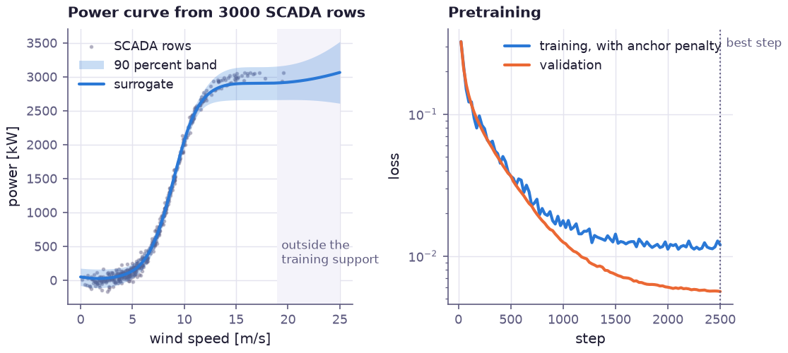
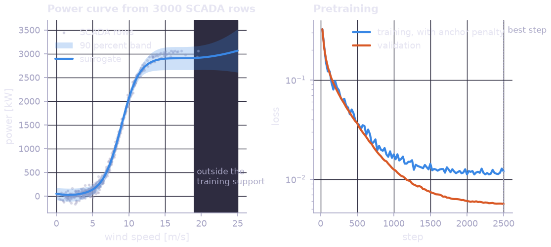
A turbine power curve learned from 3000 SCADA rows by a free-tier network of three dense layers. The band combines the spread of five anchored ensemble members with the residual noise, and the shaded region lies outside the training support, where the support guard flags every query. A monotone layer (licensed) and a bounded output layer can additionally make the curve increase with wind speed and stay below the rated power by construction.

Why a surrogate inside the graph

Most learned surrogates live outside the model that uses them: a network is trained, frozen, and called. prophys keeps it inside, which gives four things a stand alone network cannot:

• Joint fitting. The surrogate’s weights are Param leaves. The same gradient that calibrates an emission rate or a copula correlation also moves the surrogate, so outcome data correct a biased simulator.

• Controlled feedback. The pretrained posterior becomes a prior, and a single dial chooses between keeping the surrogate fixed (cut feedback), full joint estimation, and trusting the outcome data more than the pretraining data.

• Uncertainty that propagates. What the surrogate does not know enters the Monte Carlo draw as a random variable, so tail risk, Sobol indices and Shapley attributions include it.

• Structure that survives training. Monotone, convex, Lipschitz and bounded layers keep their guarantee through pretraining and fine tuning because the guarantee is architectural, not a penalty.

All numerics run in the optimized native kernels, on the CPU and on the GPU with identical bits. See Performance for timings against TensorFlow, PyTorch and XLA.

Quick start

import prophys as prp
from prophys import nn

# a surrogate with unit checked inputs and output
power = nn.Surrogate("power", {"v": "m/s", "rho": "kg/m^3"}, "kW", hidden=(64, 64))

# pretrain on its own data
report = nn.pretrain(power, {"v": v_scada, "rho": rho_scada}, p_scada)
print(report)              # R2, CRPS, interval coverage, diagnostics

# use it in a model like any expression
wind = prp.RandomVariable("wind", prp.Weibull(scale=prp.Param("A", init=8.0), concentration=2.0))
energy = prp.UncertainAttribute("energy", prp.Gaussian(power(wind, 1.225), 50.0), unit="kW")
model = prp.ProbabilityModel(energy).compile(n_samples=4000)

# fine tune everything against metered energy, anchored to the pretraining
fit = prp.finetune(model, {"energy": metered}, surrogate_feedback=1.0)
fit.surrogate_shift(power)   # how far the outcome data moved it, in nats

Configuration

A surrogate is described by its inputs, its outputs and its layers.

Argument	Meaning
inputs	Input names, or a mapping from name to unit string. Calls accept (expr, unit) pairs and convert them, and incompatible units are refused.
output / outputs	One output unit, or several named outputs (a list, or a mapping from name to unit). s.named(...) returns one node per output.
hidden and activation	Shortcut for a stack of dense layers.
layers	An explicit layer list. A linear output layer of the output width is appended when the stack does not already end in a head.
monotone	Input name to +1 or -1. Every layer is then checked to preserve monotonicity.
standardize	Input and output standardisation, set from the data by pretrain.
members	Anchored ensemble members, evaluated in one kernel call.

# two named outputs with units, three hidden layers
turbine = nn.Surrogate("turbine", {"v": "m/s", "ti": ""}, outputs={"power": "kW", "thrust": "kN"},
                       hidden=(128, 128, 64), activation="gelu")
nodes = turbine.named(wind, 0.1)       # {"power": ..., "thrust": ...}

# explicit layers and a structural guarantee
hazard = nn.Surrogate("hazard", ["age", "load"], "1/yr",
                      layers=[nn.Monotone(32, "softplus"), nn.Monotone(32, "softplus"),
                              nn.Monotone(1, output=True), nn.Positive()],
                      monotone={"age": +1, "load": +1})

Layer catalogue

Layer	What it does	Tier
Dense(width, activation, lora_rank=0)	Affine map and activation (identity, relu, leaky relu, silu, tanh, sigmoid, softplus, gelu, sin, elu). With lora_rank the base weight is frozen and a low rank update trains (LoRA).	free, LoRA licensed
Residual(activation, depth)	h + f(h) with depth dense layers inside.	free
Fourier(features, scale)	Random or learned Fourier features for smooth and periodic inputs.	free
RFF(features, lengthscale)	Random Fourier features of an RBF kernel with learned length scale. A linear head on top is a sparse spectrum Gaussian process.	free
LayerNorm(), Activation(name), Positive()	Normalisation and elementwise maps.	free
Bounded(low, high)	Sigmoid into an interval in output units.	free
Choice(temperature)	Softmax over alternatives, a differentiable discrete choice model for behavioural responses.	free
Monotone(width, activation)	Constrained monotone layer (Runje and Shankaranarayana 2023), universal monotone approximator that extrapolates trends.	licensed
InputConvex(widths, outputs)	Input convex network (Amos et al. 2017), convex in every input.	licensed
Lipschitz(width, activation, cap)	Row sums of the weight bounded by cap, with s.lipschitz_bound() in raw units.	licensed
QuantileHead(levels)	Non crossing quantiles, trained with the pinball loss.	free
HistogramHead(bins, borders, tails)	Bin probabilities of a bar distribution with exponential tails, see Probabilistic Training.	free
GaussianHead(), MixtureHead(k)	Heteroscedastic Gaussian and Gaussian mixture likelihoods.	free
Physics(fn)	A layer whose body is a prophys expression, see Physics layers and physics informed training.	free
SelfAttention, CrossAttention, PoolAttention, PrefixAttention, SliceAttention, TransolverBlock, SetBlock	Attention over sets and fields, see Field surrogates and distributions as inputs.	licensed
PoolMean(), Reshape(rows, cols)	Set pooling and reshaping.	free

Every weight follows the PyTorch Linear layout, so state dictionaries convert without transposes (prophys.nn.load_state_dict()).

Pretraining

prophys.nn.pretrain() trains a surrogate on its own data before it enters a model.

report = nn.pretrain(
    s, inputs, targets,
    loss=None,              # mse, mae, bce, crossentropy, poisson, pinball, gaussian, mixture,
                            # hl_gauss, histogram_ce, kl, crps, beta_nll, or a {name: weight} mix
    target_kind="value",    # or samples, probs, cdf
    val_fraction=0.2,
    n_steps=2000, learning_rate=3e-3, batch_size=256, weight_decay=0.0,
    residuals=(),           # physics informed residuals
    patience=None,          # early stopping on the validation loss
)

It standardises inputs and targets from the training split, trains with AdamW and a cosine schedule, keeps the weights with the best validation loss, and then stores on the surrogate everything the later stages need.

Stored in s.pretrained	Content
card	The PretrainResult: RMSE, MAE, R2, CRPS, interval coverage, noise level, data hash, history and diagnostics.
posterior	Laplace posterior of the linear head (the leaves of trees), with the prior precision chosen by maximising the evidence on a fixed grid.
support	The training support, a quantile box and a shrunk Mahalanobis ellipsoid.
prior	Diagonal Gauss Newton precision of every weight, estimated with Rademacher probes, the anchor for fine tuning.

The training is checked while it runs. Convergence is judged from the loss slope per unit step size at the start and the end of the run, which keeps the decaying schedule from hiding unfinished training. The report lists every finding with a code, see Diagnostics.

warning[NN201] the loss still falls at 86 percent of its initial rate per unit step size
  --> surrogate 'power'
   = hint increase the number of steps or the learning rate

Heads and uncertainty

A linear head gives a point prediction with an exact Laplace posterior. Probabilistic heads give a predictive distribution:

q = nn.Surrogate("load", ["v"], layers=[nn.Dense(64, "silu"), nn.QuantileHead((0.05, 0.5, 0.95))])
nn.pretrain(q, v, load)
dist = q.distribution(wind)            # a prophys Distribution
attr = prp.UncertainAttribute("load", dist)

QuantileHead defines a distribution whose quantile function is piecewise linear through the predicted quantiles, so its density, CDF, mean and reparameterised samples are closed form. GaussianHead and MixtureHead give a Gaussian and a Gaussian mixture. Beyond the outer levels the quantile head has exponential tails (see Probabilistic Training); HistogramHead gives a bar distribution.

The epistemic uncertainty of the surrogate enters a model through s.epistemic(...). It adds a random variable named <surrogate>/epistemic: a standard normal scaled by the Laplace predictive standard deviation for a linear head, or a uniform member index for an ensemble. Monte Carlo statistics then average over what the surrogate does not know, and sensitivity analyses report its share.

energy = prp.UncertainAttribute("energy", prp.Gaussian(power.epistemic(wind, 1.225), 50.0))
prp.sobol_sensitivity(model, "energy").first_order   # includes "power/epistemic"

Extrapolation guard

s.in_support(...) is one inside the training support and zero outside, and s.support_distance(...) is the distance relative to the support boundary. Both are ordinary nodes, so a model can report the probability that its surrogate is extrapolating, or gate it.

inside = prp.UncertainAttribute("inside", prp.Gaussian(power.in_support(wind, 1.225), 1e-6))
share_inside = prp.ProbabilityModel(inside).compile(n_samples=4000).expectation("inside")

Physics layers and physics informed training

A Physics layer is written with ordinary prophys operations over the columns it receives, and may hold its own Param leaves. A network can be “physics in the middle, learned residuals around it” (a universal differential equation style model) or “physics as a feature extractor”.

Expressions built from elementary operations compile into the native program itself. The physics becomes a register program inside the network interpreter, with exact first and second derivatives, the same bits on CPU and GPU, and one export blob for the runtime. Its Param leaves keep their names and transforms and train with the weights. Pretraining applies weight decay to network weights only, so a physical constant is never pulled toward zero.

Operations that compile natively

Group	Operations
arithmetic	+ - * /, negation, powers (constant or learned exponent)
elementary	exp log log10 sqrt sin cos tan tanh, deg2rad rad2deg
smooth	softplus sigmoid erf erfc
piecewise	abs sign relu clip maximum minimum, where over comparisons
leaves	layer columns, constants, scalar Param and elements of vector Param

Anything else, such as a Green’s function or a norm, runs as a prophys stage between the native segments. The surrogate still trains and evaluates, surrogate.python_physics lists the reason per layer, and export raises NN112. nn.Physics(fn, native=True) turns that fallback into an error at build time.

k = prp.Param("drag", init=0.4, transform="softplus")
s = nn.Surrogate("hybrid", ["v", "rho"], layers=[
    nn.Physics(lambda v, rho: [0.5 * rho * v**3 * k, v]),   # aerodynamic power and speed
    nn.Dense(32, "silu"),
    nn.Dense(1, "identity"),                                # learned correction
])

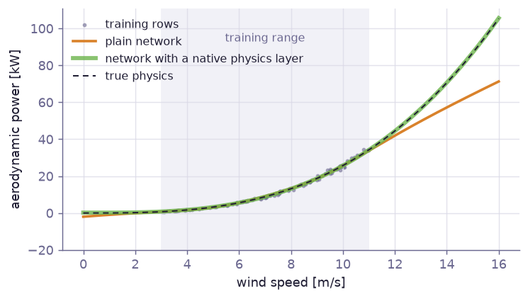
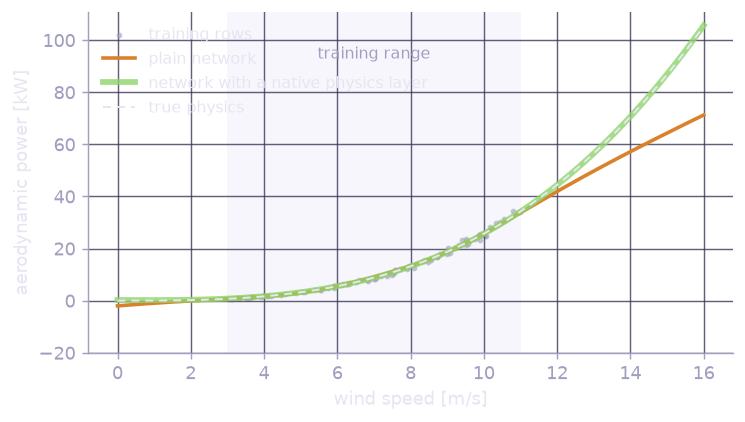
Trained on wind speeds between 3 and 11 m/s. The plain network bends away outside that range, the network whose physics layer carries the cube law follows it and learns the drag coefficient.

Physics informed training adds residuals of differential equations to the pretraining loss. Derivatives are exact, computed by Taylor mode differentiation inside the native interpreter (first and second directional derivatives in one pass, and their gradients with respect to every weight):

# u' + u = 0 with u(0) = 1
res = nn.PhysicsResidual(lambda D: D.d("t")[:, 0] + D.u[:, 0], t_collocation)
nn.pretrain(s, t0, u0, residuals=[res])

Derivatives offers u, d(i), dd(i), laplacian(...) and input(i) by input index or name.

Field surrogates and distributions as inputs

A FieldSurrogate takes a set of rows, one row per token. Token helpers turn prophys structures into rows:

Helper	Rows
field_tokens(field)	One per raster cell, centre coordinates and values.
point_tokens(points, features)	One per point, coordinates and features.
geometry_tokens(geometry)	One per segment or polygon edge.
sample_set(expr, n)	n fresh Monte Carlo draws of any expression, drawn with common random numbers so they are smooth in the model parameters.

sample_set makes the surrogate a map from a distribution to an output: the input is the empirical distribution of an upstream quantity, not one value of it.

gust = prp.RandomVariable("gust", prp.Weibull(scale=prp.Param("gust_scale", init=10.0), concentration=2.2))
damage = nn.FieldSurrogate("damage", rows=256, cols=1,
                           layers=[nn.Dense(64, "gelu"), nn.SetBlock(heads=4), nn.PoolAttention(4), nn.Dense(1)])
node = damage(nn.sample_set(gust, 256))

Physics attention of Transolver (Wu et al. 2024) handles irregular meshes in time linear in the number of points, and cross attention reads geometry or sensor context:

wake = nn.FieldSurrogate("wake", rows=1024, cols=3, context=(64, 4), layers=[
    nn.Dense(64, "gelu"),
    nn.TransolverBlock(heads=4, slices=32),
    nn.CrossAttention(heads=4),
    nn.TransolverBlock(heads=4, slices=32),
    nn.Dense(1, "identity"),
])
deficit = wake(nn.field_tokens(inflow), nn.geometry_tokens(farm_layout))

Pretrained Transolver weights load from a PyTorch state dictionary:

nn.load_state_dict(wake, torch_model.state_dict(), nn.transolver_mapping("L1", "blocks.0"))

Neural operators: DPOT

DPOT (Hao et al. 2024) is a Fourier neural operator pretrained on many PDE datasets. It reads in_timesteps snapshots of a field on an X by Y grid and predicts the next out_timesteps. prophys builds the same network on the native interpreter, so a released checkpoint fine tunes, runs inside a model and exports to the runtime like any other surrogate.

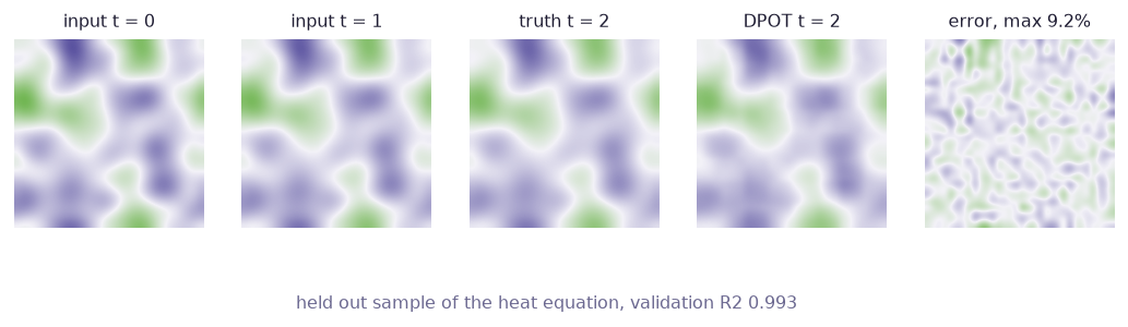
A small DPOT trained from scratch on the periodic heat equation, predicting the third snapshot of a held out sample from the first two.

# a new operator
op = nn.DPOT("flow", grid=(128, 128), in_channels=4, in_timesteps=10, patch_size=8,
             embed_dim=512, depth=6, n_blocks=8, modes=32, normalize=True)

# or a released checkpoint, its shape is read from the tensors
state = torch.load("model_Ti.pth", map_location="cpu")["model"]
op = nn.from_dpot(state, modes=32, out_timesteps=1)

tokens = nn.dpot_tokens(fields)                  # [..., X, Y, T, C] to [..., X Y T, C]
nn.pretrain(op, tokens, next_fields.reshape(n, -1, 4))
pred = op.fields(op.apply(None, tokens))         # back to [..., X, Y, out_timesteps, C]

The network consists of eleven native operations: channel statistics for the normalisation and its inverse, the coordinate grid, patch embedding, the position table, the time aggregation of DPOT, AdaIN scaling, group norm, the adaptive Fourier mixer (rfft2, a block diagonal complex MLP on the kept modes and irfft2), transposed patch convolution and denormalisation. Each has an exact reverse pass and Taylor mode derivatives, runs the same numerics on CPU and GPU, and matches the PyTorch reference to double precision round off in the forward pass and in every gradient. Parameter names follow the PyTorch module (blocks/3/filter/w1), so nn.dpot_state converts any checkpoint by name and checks every shape. The classification head of the reference is not built.

Physics layers and fine tuning work as for any surrogate. A field observation of a quantity downstream of the operator trains, for example, only the output layers with trainable=["flow/L0/out_layer/*"]. The time aggregation and the Fourier mixer are licensed features.

Tree ensembles

TreeEnsemble is a sum of complete axis aligned trees whose splits are softsign relaxations (GRANDE, Marton et al. 2024). In evaluation mode they route hard exactly as XGBoost does, in optimisation mode they train with straight through gradients (hard forward, softsign backward), so the trained ensemble is the hard ensemble it deploys as.

trees = nn.TreeEnsemble("rail_break", {"temp": "degC", "traffic": "1/d", "age": "yr"}, "1/km/yr",
                        n_trees=200, depth=4, monotone={"age": +1})
nn.pretrain(trees, records, breaks)          # projection keeps monotonicity after every step

# or start from a trained booster
trees = nn.TreeEnsemble.from_xgboost(booster, inputs=["temp", "traffic", "age"])
trees = nn.TreeEnsemble.from_lightgbm(lgb_booster, inputs=[...])

Imported boosters reproduce their predictions to single precision rounding, keep their node covers for exact TreeSHAP, and fine tune inside the model like any other surrogate.

Fine tuning inside the model

prophys.finetune() accepts two surrogate options.

surrogate_feedback

The power of the pretrained posterior used as prior, per surrogate or for all. 0 keeps the surrogate at its pretrained weights, 1 is joint estimation of pretraining and outcome data, values above one discount the pretraining data (a simulator known to be biased).

surrogate_scope

head trains the final linear layer (the leaves of trees) and every physical parameter, all trains every surrogate weight.

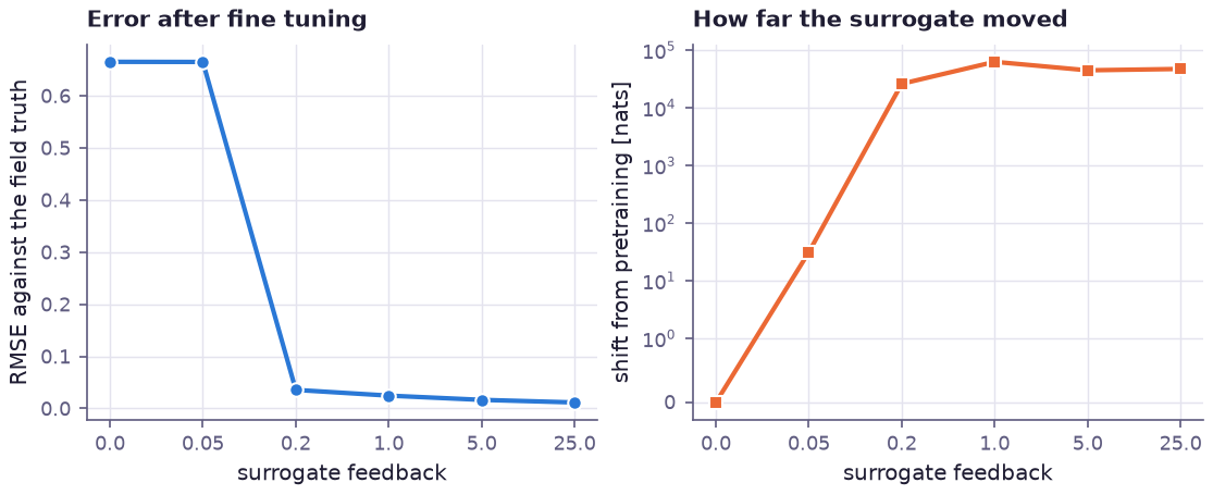
A surrogate pretrained on a simulator with a 20 percent bias, fine tuned against 150 field observations. Cutting the feedback keeps the simulator bias, larger feedback lets the outcome data correct it. The shift from the pretrained posterior is reported in nats by CalibrationResult.surrogate_shift.

Export and runtime

Model packages of format 1.2 include every surrogate of the model with its program or tree spec, weights, support region, head posterior, training card and a parity checksum. The prophys-runtime library evaluates them without Python through a C interface, with the same interpreter and therefore the same bits, see Runtime Library. Surrogates with native physics layers export like any other network.

Performance

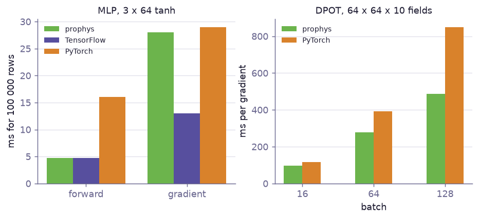
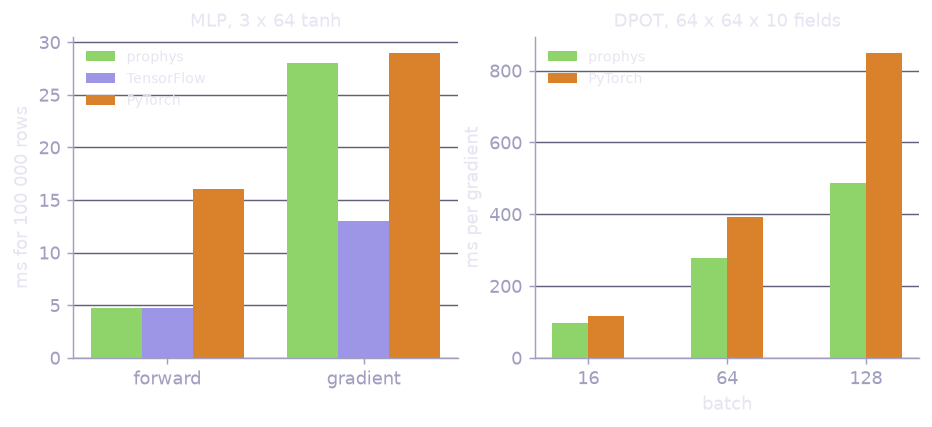
The interpreter runs single precision buffers (JAX’s default) in single precision with fused multiply add in dense layers, and double precision buffers in double precision. On the CPU, sixteen samples travel together in one SIMD lane pack, and gradients are reduced in a fixed blocked order that the GPU kernels follow as well. Measured for a four input network with three hidden tanh layers of 64 units on an Apple M series CPU (seconds, lower is better):

Batch	prophys forward	TensorFlow forward	XLA forward	PyTorch forward	prophys gradient	TensorFlow gradient	PyTorch gradient
1 000	0.00011	0.00030	0.00026	0.00023	0.00068	0.00044	0.00046
100 000	0.0047	0.0047	0.0054	0.016	0.028	0.013	0.029
1 000 000	0.046	0.046	0.051	0.16	0.20	0.13	0.29

The forward pass matches TensorFlow, and the gradient, which also computes exact reproducible per block reductions, is within a factor of two of it and faster than PyTorch.

Large programs such as neural operators switch to packs of four samples, so even a batch of sixteen spreads over several cores, and their weight gradients are summed over blocks of rows before they reach the accumulator. For a DPOT on 64 by 64 fields with ten input steps, 128 channels and four blocks, measured against the PyTorch reference with all threads:

Batch	prophys forward	PyTorch forward	prophys gradient	PyTorch gradient
16	0.024	0.062	0.097	0.116
64	0.060	0.220	0.277	0.392
128	0.119	0.451	0.487	0.850

Determinism

Every result is a fixed function of its inputs. The same interpreter code runs on the CPU in lane packs and on the GPU one sample per thread, elementary functions are written with plain IEEE arithmetic, fused multiply add is correctly rounded on every platform, and gradient sums follow one canonical order. Parity tests run every kernel on an emulated device and compare it with the CPU bit for bit.

Licensing

Surrogates within the free tier run without a license: networks with at most four weighted layers built from the free layers, and tree ensembles of at most 20 trees of depth 4 without learned split features. Attention, LoRA, monotone, input convex and Lipschitz layers, larger networks and larger ensembles need a license. The check runs inside the native kernels, and a surrogate beyond the free tier warns at construction (LIC101). See License.