

Example: Fast-Charge Thermal Risk with a Learned Surrogate#
A fleet operator wants to raise the fast-charge rate of a 96 cell battery
pack. The cell datasheet allows charging up to 45 °C, so the decision rests
on the probability that the hottest cell exceeds that limit during a charge
from 10 to 80 % state of charge, given what varies in the field: the coolant
inlet temperature, the flow of an ageing pump and the resistance growth of
ageing cells. The peak cell temperature comes from an electro-thermal
simulator that is too slow to call inside a Monte Carlo loop over 96 cells,
so a learned surrogate replaces it. The surrogate carries the known physics
in a Physics layer, is pretrained on simulator rows
with pretrain(), and then becomes an ordinary node of a
ProbabilityModel: its own uncertainty is a random
input, its training support is checked on every draw, it is fine tuned
against fleet telemetry with finetune(), the tail
risk is attributed with shapley_effects(), and the
fine tuned network is exported for the battery management system. Every
surrogate stays on the free tier. The full runnable source is
examples/learned_surrogate/model.py.
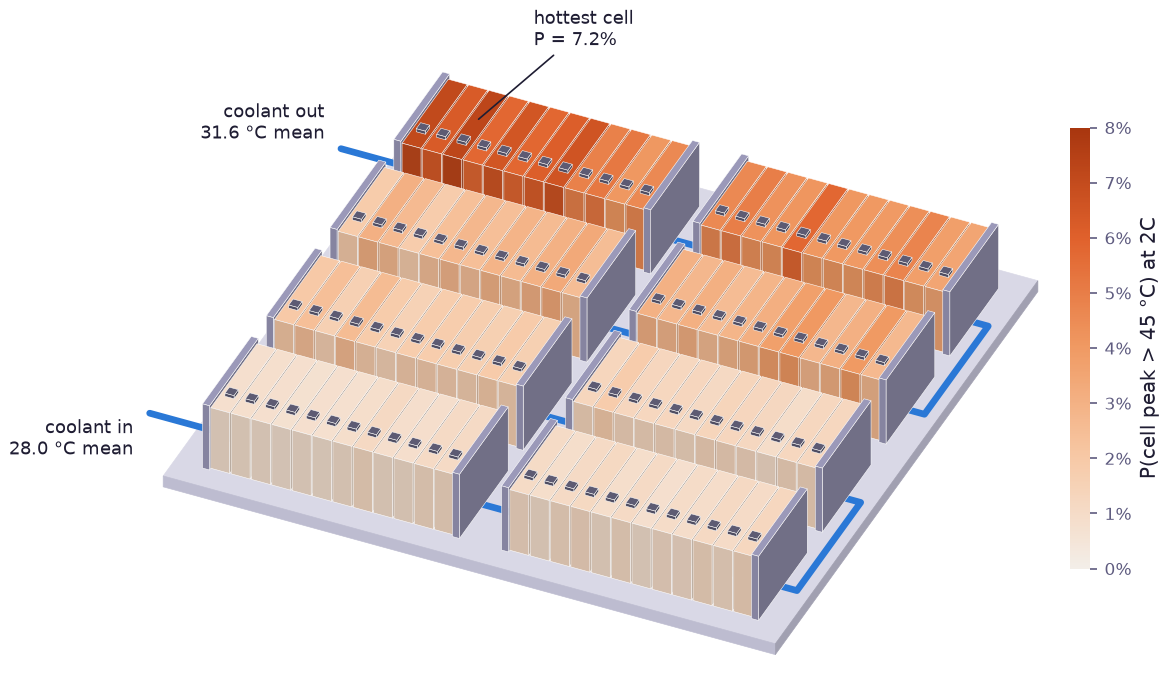
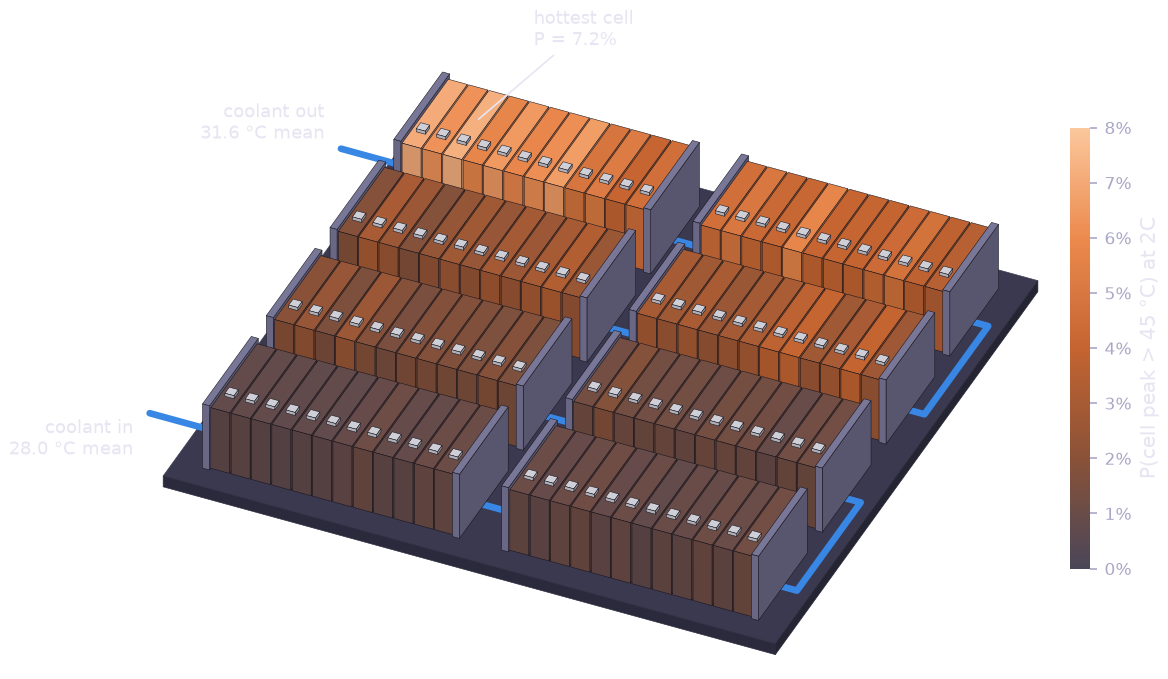
The pack: eight modules of twelve prismatic cells on one cold plate, with the coolant loop running under the modules from the front left to the back left. Each cell is coloured by the probability that its peak temperature exceeds 45 °C during a 2C charge, computed with the fine tuned surrogate over 4 000 draws of the operating conditions. The coolant picks up the heat of every cell it passes, 3.6 K on average, so the risk grows along the loop from under 1 % at the inlet to 7.2 % at the hottest cell near the outlet, where the end-of-line resistance spread adds cell-to-cell differences.
Step 1 — The simulator and its training rows#
The reference model is a two-node thermal model of a 50 Ah cell (core and can, Lin et al. 2014) with Joule heat \(q = I^2 R(T, \mathrm{soc})\). The resistance follows an Arrhenius law in the core temperature and rises at low and high state of charge, and the cold-plate conductance scales with the coolant flow to the power 0.8 (Dittus–Boelter). The model is integrated over the constant-current phase in JAX and returns the peak core temperature:
def rhs(tc, ts, t):
    soc = SOC_START + (SOC_END - SOC_START) * t / t_end
    r = r_cell * 1e-3 * jnp.exp(E_ACT / R_GAS * (1 / (tc + 273.15) - 1 / 298.15)) * soc_factor(soc)
    q = heat_factor * current**2 * r
    return (q - (tc - ts) / R_CORE) / C_CORE, ((tc - ts) / R_CORE - (ts - t_cool) / r_ext) / C_SURF
It is sampled on a box of 2 400 operating points:
INPUTS = {"c_rate": "h^-1", "t_cool": "degC", "flow": "L/min", "r_cell": "mV/A"}
BOX = {"c_rate": (0.5, 3.0), "t_cool": (10.0, 45.0), "flow": (2.0, 10.0), "r_cell": (0.7, 1.6)}
N_TRAIN = 2400

_rng = np.random.default_rng(0)
train_x = {k: _rng.uniform(lo, hi, N_TRAIN) for k, (lo, hi) in BOX.items()}
train_y = np.asarray(simulator(*train_x.values()))
The input units are declared, so a call with a coolant temperature in kelvin or a resistance in ohm is converted or refused.
Step 2 — Physics inside the network#
With constant heat the two-node model is linear and has a closed-form
solution: two exponentials whose rates are the eigenvalues of a 2 by 2
matrix. two_node_rise writes that solution with prophys operations and
corrects the resistance for temperature with four damped fixed-point
steps. On its own it follows the simulator with an RMSE of about 0.5 K.
The physics layer
passes its estimate to the network together with the scaled inputs:
def physics_features(c_rate, t_cool, flow, r_cell):
    """Physics estimate of the peak temperature and the scaled inputs."""
    estimate = t_cool + two_node_rise(c_rate, t_cool, flow, r_cell)
    return [
        (estimate - 35.0) / 10.0,
        (c_rate - 1.75) / 0.75,
        (t_cool - 27.5) / 10.0,
        (flow - 6.0) / 2.3,
        (r_cell - 1.15) / 0.26,
    ]


# Physics layer, then h + f(h) with two dense layers inside, then the
# linear head: the physics estimate reaches the head unchanged, the network
# learns the correction. Four weighted layers, on the free tier.
cell = nn.Surrogate(
    "cell",
    INPUTS,
    "degC",
    layers=[nn.Physics(physics_features), nn.Residual("silu", depth=2, width=32), nn.Dense(1, "identity")],
)

# Two baselines without physics, for comparison only.
plain = nn.Surrogate("plain", INPUTS, "degC", hidden=(32, 32))
trees = nn.TreeEnsemble("trees", INPUTS, "degC", n_trees=20, depth=4)
The expression uses only elementary operations, so it compiles into the
native network program: the surrogate stays a single program with exact
derivatives that exports like any other network. The
Residual block starts close to the identity, so the
physics estimate reaches the linear head directly and the two inner layers
learn what the closed form misses: the state-of-charge profile of the
resistance and the error of the approximate temperature correction. Pretraining is one call
per surrogate:
cards = {
    "cell": nn.pretrain(cell, train_x, train_y, n_steps=3000, learning_rate=5e-3),
    "plain": nn.pretrain(plain, train_x, train_y, n_steps=1500, learning_rate=5e-3),
    "trees": nn.pretrain(trees, train_x, train_y, n_steps=1000, learning_rate=3e-2),
}
Each card reports the validation RMSE, R2, interval coverage and the
convergence findings. pretrain() also stores on the
surrogate its training support (a quantile box and a Mahalanobis
ellipsoid), the Laplace posterior of its linear head and the prior used
later for fine tuning.
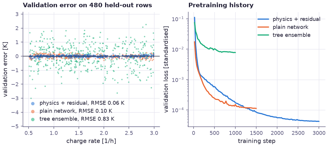
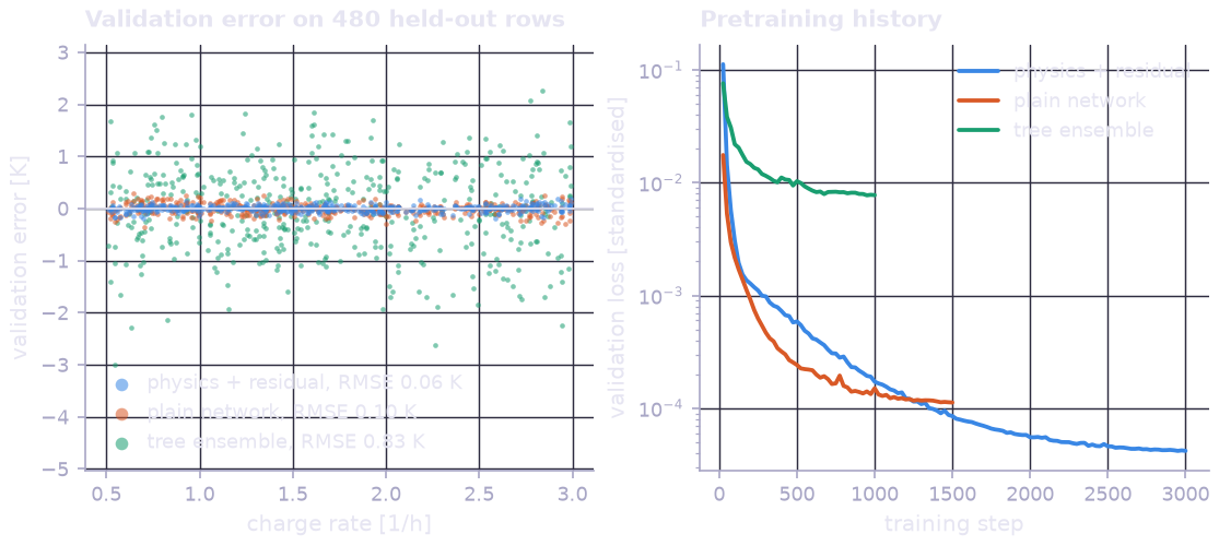
Left: error of the three surrogates on the 480 validation rows that
pretraining holds out. Both networks stay within a few tenths of a kelvin,
the 20 trees of depth 4 within about 3 K. Right: the validation loss during
pretraining. The tree ensemble reports NN201 (its splits are still
moving when training stops), which is acceptable for a baseline.
Inside the training box both networks are accurate. The difference shows beyond it:
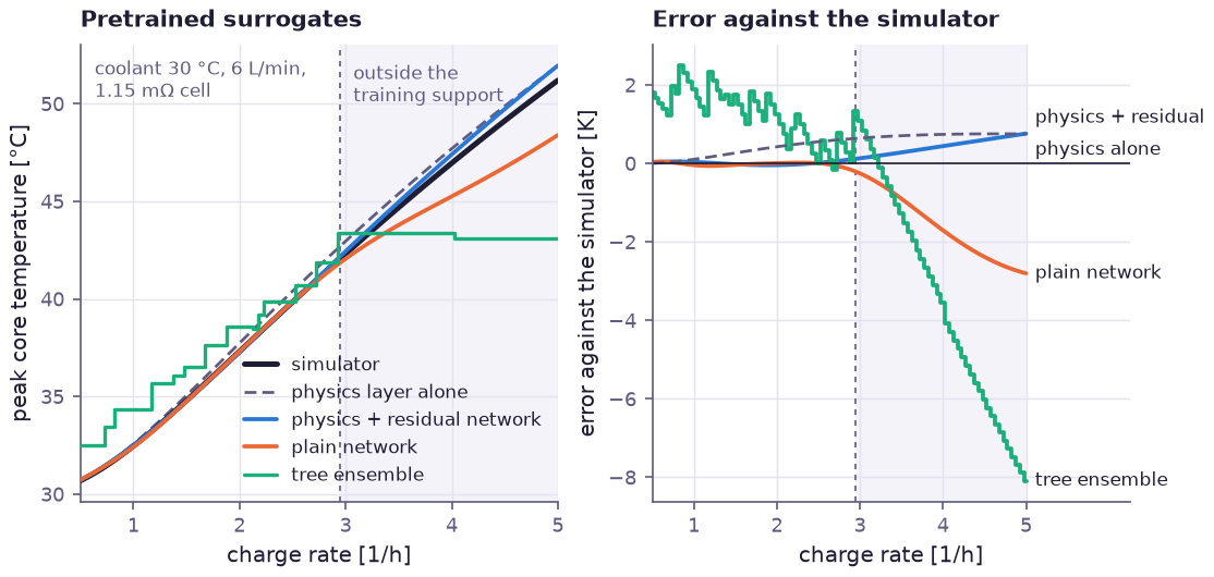
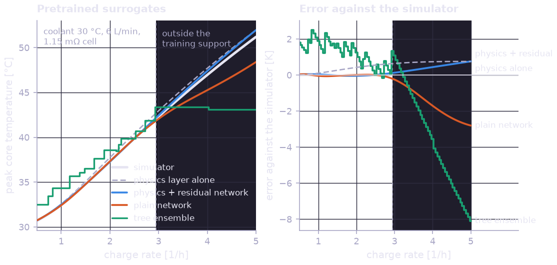
The peak temperature against the charge rate at one operating point, for the simulator, the physics layer alone and the three pretrained surrogates. Training stopped at 3C (shaded region beyond). The tree ensemble is piecewise constant and flat outside its data, 8 K low at 5C. The plain network bends away and is 2.8 K low. The surrogate with the physics layer follows the simulator to within 0.8 K, because the closed form carries the trend into the region where there are no training rows.
Step 3 — The pack as a probability model#
The pack has eight modules of twelve cells in series along one coolant
loop. The coolant temperature at each cell follows from an energy balance
over the cells upstream of it, the resistance of each cell is its measured
end-of-line spread times the fleet’s ageing factor, and the operating
conditions are random variables. The charge rate is the decision, a
Param:
# Uncertain operating conditions of a fast charge in the hot season.
t_inlet = prp.RandomVariable("t_inlet", prp.Gaussian(28.0, 4.0))  # coolant inlet [degC]
flow = prp.RandomVariable("flow", prp.LogNormal(mu=float(np.log(6.0)), sigma=0.2))  # [L/min]
ageing = prp.RandomVariable("ageing", prp.LogNormal(mu=float(np.log(1.15)), sigma=0.08))  # resistance growth

# The charge rate is the decision.
c_rate = prp.Param("c_rate", init=2.0)

current = c_rate * CAPACITY
r_cells = R_NEW * ageing * cell_spread[:, None]  # (96, n) [mOhm]
# Energy balance of the coolant (DC-resistance heat at 25 degC, averaged over the charge).
mass_flow_heat = flow / 60000.0 * RHO_CP  # [W/K]
t_cool_cells = t_inlet + current**2 * R_NEW * 1e-3 * SOC_MEAN_FACTOR * ageing * upstream_heat / mass_flow_heat
The surrogate is called like any expression. Its inputs broadcast to 96 cells by the Monte Carlo draws, and the attribute is the hottest of them:
peak_cells = cell(c_rate, t_cool_cells, flow, r_cells)  # (96, n) [degC]
peak_cells_epistemic = cell.epistemic(c_rate, t_cool_cells, flow, r_cells)

THERMISTOR_SIGMA = 0.3  # [K]
hottest = prp.UncertainAttribute(
    "hottest_cell",
    prp.Gaussian(_hottest(peak_cells_epistemic), THERMISTOR_SIGMA),
    unit="degC",
    domain="peak temperature of the hottest cell during a fast charge",
)
inside = prp.UncertainAttribute(
    "inside_support",
    prp.Gaussian(_all(cell.in_support(c_rate, t_cool_cells, flow, r_cells)), 1e-6),
    domain="one when every cell's operating point lies inside the training support",
)
pack_model = prp.ProbabilityModel(hottest, inside)
cell.epistemic adds the random variable cell/epistemic, a standard
normal scaled by the Laplace predictive standard deviation of the linear
head, so every Monte Carlo statistic averages over what the surrogate does
not know. cell.in_support is one where an operating point lies inside
the training support, and inside_support is the share of draws in which
all 96 cells do.
Step 4 — Fine tuning against the fleet#
Telemetry from 80 fast charges logs the operating point and the peak temperature of a monitored cell. The simulator assumed the DC-resistance Joule heat, but at high current the effective heat is 25 % higher, so the pretrained surrogate reads 1.4 K low on average, more at high rates. The surrogate enters a second model at the logged operating points, with a learned noise level:
field_sigma = prp.Param("field_sigma", init=0.5, transform="softplus")
field_peak = prp.UncertainAttribute(
    "field_peak",
    prp.Gaussian(cell(*(jnp.asarray(v) for v in field_x.values())), field_sigma),
    unit="degC",
    domain="logged peak temperature of the monitored cell",
)
field_model = prp.ProbabilityModel(field_peak)
finetune() then trains the linear head against the
telemetry, anchored to the pretrained posterior raised to the power
1 / surrogate_feedback:
field = field_model.compile()
fits = {}
for fb in FEEDBACKS:
    fits[fb] = prp.finetune(
        field,
        {"field_peak": field_obs[None]},
        surrogate_feedback=fb,
        surrogate_scope="head",
        n_steps=400,
        learning_rate=2e-2,
    )
The pretraining rows are noise-free simulator output, so their posterior is
far tighter than anything 80 thermistor readings can say. With feedback 1
(joint estimation) the simulator wins and the bias stays. Only when the
pretraining data are discounted strongly does the telemetry correct the
head, and the fit is then as good as the thermistor noise allows. The fits
at feedback 100 and 1 000 report CAL201: the anchor makes them slow,
and they are shown only to trace the dial. Both models share the surrogate’s
leaves by name, so the fitted values are passed to the pack model as
parameters.
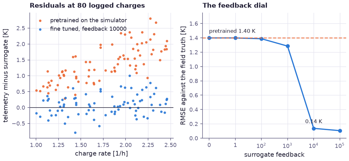
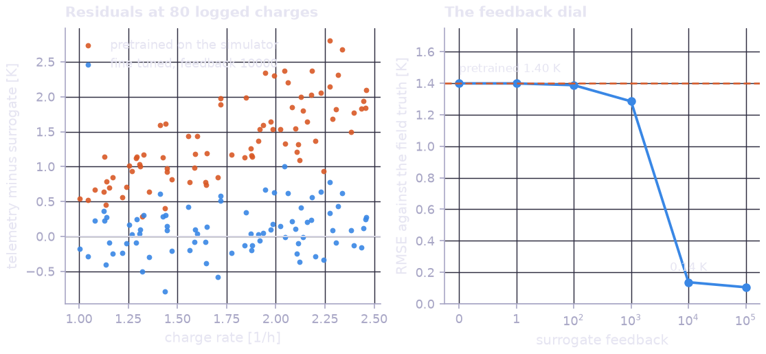
Left: telemetry minus surrogate at the 80 logged charges. The pretrained surrogate underestimates every charge, by more at higher rates where the missing heat matters most. After fine tuning the residuals centre on zero with the spread of the thermistor. Right: RMSE against the field truth on 400 fresh operating points as the feedback grows. The pretrained posterior holds the surrogate at the simulator up to a feedback of about 1 000.
Step 5 — Risk, attribution and the charge rate#
At 2C the pretrained surrogate gives a 3.6 % probability that the hottest cell exceeds 45 °C, and the fine tuned one 8.0 %. The support guard reports that 99.1 % of the draws lie inside the training support, so this is an interpolation.
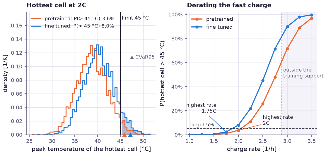
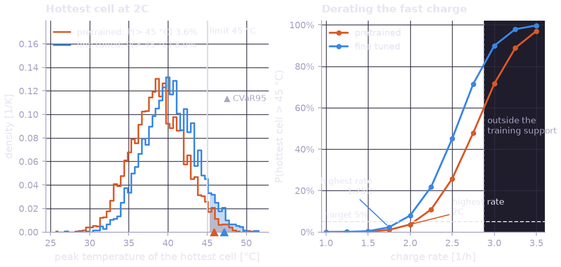
Left: the peak temperature of the hottest cell at 2C, with the pretrained and the fine tuned surrogate. The shaded tails lie beyond the 45 °C limit and the triangles mark the CVaR95, 45.9 °C and 47.2 °C. Right: the exceedance probability over the charge rate. The fine tuned model meets the 5 % target up to 1.75C, the simulator alone would have allowed 2C. Beyond 2.75C no draw lies entirely inside the training support (shaded), and the exceedance there is an extrapolation.
Shapley effects attribute the variance and the tail average above the 95 % quantile to the four random inputs, the surrogate’s epistemic variable included:
attribution = {
    "variance": explain.shapley_effects(
        compiled,
        "hottest_cell",
        statistic="variance",
        n_outer=1000,
        n_inner=32,
        params={"c_rate": jnp.asarray(2.0), **tuned},
    ),
    "cvar": explain.shapley_effects(
        compiled,
        "hottest_cell",
        statistic="cvar",
        level=0.95,
        n_outer=500,
        n_inner=128,
        params={"c_rate": jnp.asarray(2.0), **tuned},
    ),
}
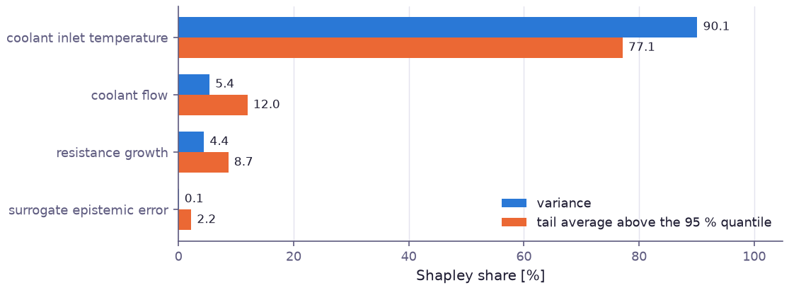
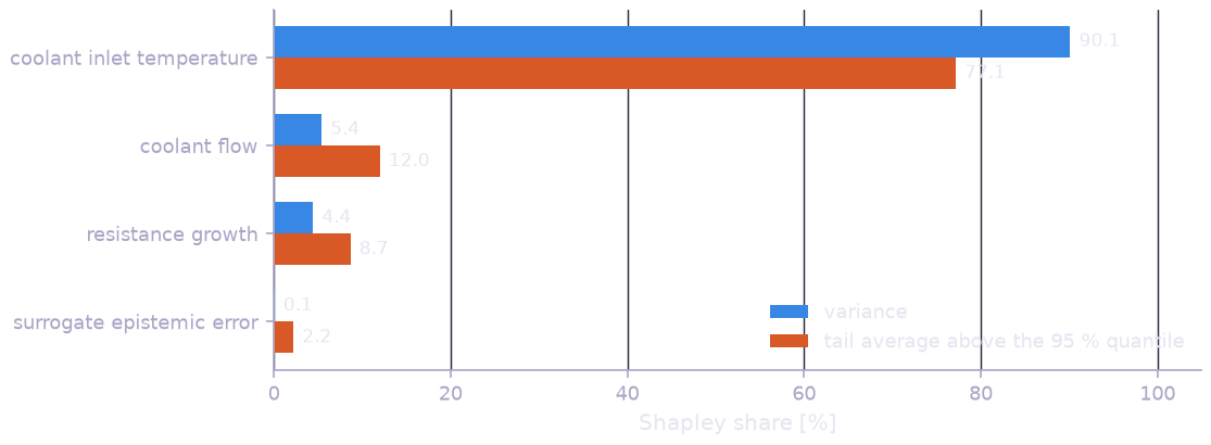
Shapley shares of the hottest-cell temperature at 2C. The coolant inlet temperature explains 90 % of the variance. The tail owes more to the coolant flow and the resistance growth, which set how much heat the cells produce and how much of it the coolant carries down the loop. The surrogate’s epistemic error explains 0.1 % of the variance. Its 2.2 % of the tail is within the Monte Carlo resolution of the tail estimate, which overstates small shares.
The three kinds of surrogate error are handled by three different tools. The epistemic error of the head is quantified and turns out negligible, because 2 400 noise-free rows pin the head down. Extrapolation is not something the head posterior can see (its standard deviation stays below 0.01 K at 5C), and the support guard reports it instead. The simulator’s bias is visible only against field data, and fine tuning corrects it.
Step 6 — Export#
The fine tuned surrogate, with its physics layer, support region, head posterior and training card, is exported for the battery management system. The parity checksum lets the runtime verify that it reproduces the same outputs:
exp = export_surrogate(cell, tuned)
Results#
The console output of python examples/learned_surrogate/model.py
(warnings omitted):
=== Pretraining on 2400 simulator rows ===
  cell   validation RMSE 0.061 K   R2 1.0000
  plain  validation RMSE 0.099 K   R2 0.9999
  trees  validation RMSE 0.825 K   R2 0.9918

=== Extrapolation to 4C (trained up to 3C), simulator 47.0 degC ===
  cell   47.4 degC   error +0.4 K
  plain  45.3 degC   error -1.7 K
  trees  43.4 degC   error -3.6 K

=== Pack at 2C, pretrained surrogate ===
  E[hottest cell] 38.8 degC   CVaR95 45.9 degC
  P(hottest cell > 45 degC) 3.65%   inside support 99.1%

=== Fine tuning on 80 telemetry rows ===
  RMSE against field truth, pretrained 1.40 K
  feedback       0: RMSE 1.40 K, noise 1.47 K, shift 0 nats
  feedback       1: RMSE 1.40 K, noise 1.47 K, shift 0.0777 nats
  feedback     100: RMSE 1.39 K, noise 1.46 K, shift 599 nats
  feedback    1000: RMSE 1.29 K, noise 1.37 K, shift 6.36e+04 nats
  feedback   10000: RMSE 0.14 K, noise 0.34 K, shift 1.03e+06 nats
  feedback  100000: RMSE 0.11 K, noise 0.31 K, shift 1.7e+06 nats

=== Pack at 2C, fine tuned surrogate ===
  E[hottest cell] 40.2 degC   CVaR95 47.2 degC
  P(hottest cell > 45 degC) 7.98%

=== Shapley attribution at 2C (fine tuned) ===
  variance t_inlet 90.1%, ageing 4.4%, flow 5.4%, cell/epistemic 0.1%
  cvar     t_inlet 77.1%, ageing 8.7%, flow 12.0%, cell/epistemic 2.2%

=== Derating to P(exceed) <= 5% ===
  rate   P(exceed) pretrained   P(exceed) fine tuned   inside support
  1.00C                0.0%                   0.0%            99.2%
  1.25C                0.1%                   0.1%            99.2%
  1.50C                0.2%                   0.4%            99.2%
  1.75C                1.0%                   2.3%            99.1%
  2.00C                3.6%                   8.0%            99.1%
  2.25C               10.9%                  21.8%            99.0%
  2.50C               25.8%                  45.1%            98.8%
  2.75C               47.9%                  71.5%            98.2%
  3.00C               71.6%                  90.0%             0.0%
  3.25C               88.9%                  97.9%             0.0%
  3.50C               97.0%                  99.7%             0.0%
  highest charge rate: 2.0C with the simulator, 1.75C after fine tuning

=== Export ===
  surrogate blob 9892 bytes, parity checksum e5f0cbfb02974386, verified True
The shift from pretraining is half the squared Mahalanobis distance of the fine tuned head under the pretrained posterior. Its large values measure how strongly the telemetry contradicts the noise-free simulator.
Primitives exercised#
Category |
Used for |
|---|---|
The cell surrogate: closed-form physics compiled into the network, a learned correction |
|
A free-tier tree baseline (20 trees of depth 4) |
|
Training on simulator rows; the card, support region, head posterior and fine tuning prior |
|
|
The surrogate’s own uncertainty as a random input; the extrapolation guard |
Coolant temperature, pump flow and cell ageing |
|
|
Correcting the simulator’s bias against fleet telemetry |
Variance and tail attribution, the epistemic variable included |
|
The fine tuned surrogate for the runtime, with a parity checksum |
Running it#
$ python examples/learned_surrogate/model.py