Example: Gust Loads and Stall Risk of a Light Aircraft

The operator of a four-seat light aircraft asks two questions about flying in low-level turbulence. How likely is a gust to stall the wing on the final approach, flown at the handbook speed of 68 kt? And how close do gust loads come to the structural limit load factor at higher speeds? Both answers depend on the lift curve of the wing, which is known only through wind-tunnel measurements of its airfoil. This chapter calibrates a lift polar with trailing-edge stall to those measurements with calibrate(), carries the fitted curve through lifting-line theory to the wing, flies the wing through a random gust field built with ornstein_uhlenbeck(), and reads off the probability of stall, the load-factor distribution across the flight envelope, and the local and global sensitivities of the stall risk. The full runnable source is examples/airfoil_loads/model.py.

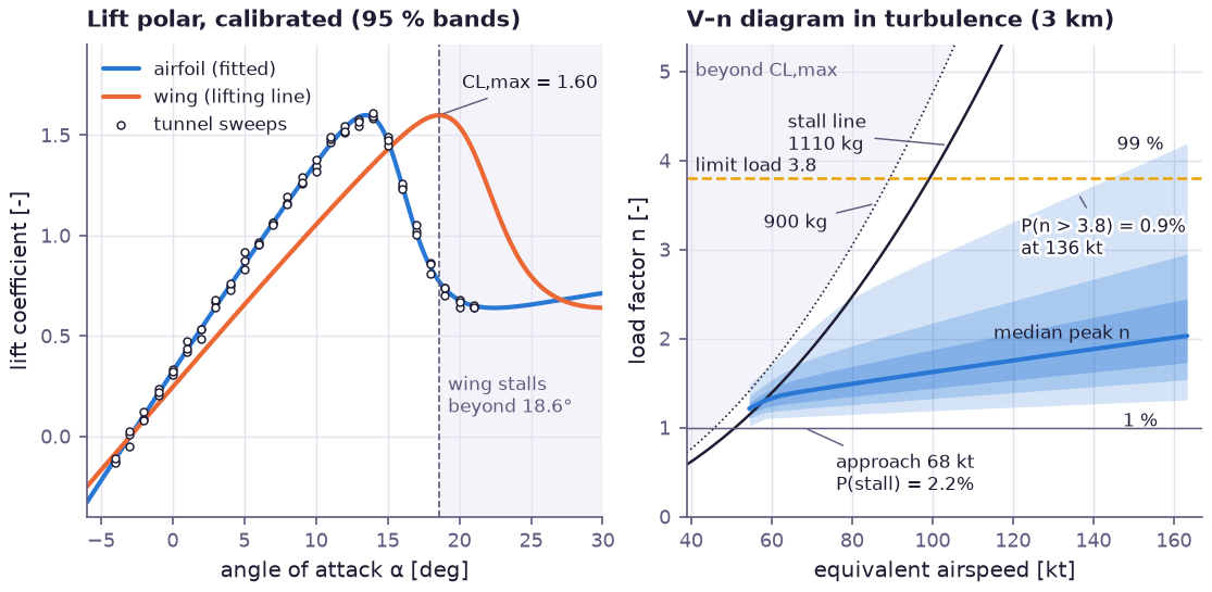
Left: the three wind-tunnel sweeps of the airfoil, the calibrated section polar and the wing lift curve that lifting-line theory derives from it, each with its 95 % band from the calibration (narrower than the lines at this scale). The wing reaches the same maximum lift as the airfoil, CL,max = 1.60, but five degrees later. Right: the V–n diagram of the aircraft in 3 km of turbulence. Above the stall lines (maximum take-off mass 1110 kg, solid; 900 kg, dotted) the wing cannot produce the load. The blue fan shows the 25–75, 10–90 and 1–99 % ranges of the peak load factor reached in the turbulence. At the approach speed the fan presses against the stall line, and 2.2 % of approaches stall; at high speed the fan widens with airspeed until its tail crosses the limit load of 3.8.

Step 1 — The lift polar, with unknown parameters

The section lift follows Kirchhoff’s flow model: the trailing-edge separation point f moves forward from the trailing edge (f = 1, attached) to the leading edge (f = 0) as a logistic function of the angle of attack, and lift falls with it. Four Param leaves describe the curve: lift slope, zero-lift angle, the angle at which the flow is separated over half the chord, and how abruptly separation spreads:

lift_slope = prp.Param("lift_slope", init=5.5, transform="softplus")  # section dCl/dalpha [1/rad]
alpha_zero = prp.Param("alpha_zero_deg", init=-1.0)  # zero-lift angle [deg]
alpha_half = prp.Param("alpha_half_deg", init=13.0)  # separation point at mid-chord, f = 0.5 [deg]
stall_width = prp.Param("stall_width_deg", init=2.0, transform="softplus")  # how abruptly f falls [deg]


def _section_cl(alpha_deg, slope, a0, a_half, width):
    """Kirchhoff lift ``Cl = slope sin(x) cos(x) ((1 + sqrt f) / 2)^2``,
    ``x = alpha - a0``, with the trailing-edge separation point ``f`` falling
    from 1 (attached) to 0 (fully separated) as a logistic function of the
    angle of attack. Linear at small angles, a rounded stall, and a
    flat-plate-like lift plateau (below Cl_max) in deep stall."""
    f = jax.nn.sigmoid(-(alpha_deg - a_half) / width)
    x = jnp.deg2rad(alpha_deg - a0)
    return slope * jnp.sin(x) * jnp.cos(x) * ((1.0 + jnp.sqrt(f + 1e-12)) / 2.0) ** 2

The finite wing (span 11 m, aspect ratio 7.5) is treated with Prandtl’s lifting-line theory for elliptic loading: the downwash lowers the effective angle of attack of every section, so the wing’s lift slope is smaller and its stall angle larger than the airfoil’s:

def _lifting_line_factor(slope):
    """Lifting-line reduction of the effective angle of attack of an
    elliptically loaded wing: ``(alpha_eff - a0) = k (alpha - a0)``,
    ``k = 1 / (1 + slope / (pi e AR))``."""
    return 1.0 / (1.0 + slope / (jnp.pi * OSWALD * ASPECT_RATIO))


def _wing_cl(alpha_deg, slope, a0, a_half, width):
    """Lift coefficient of the finite wing at geometric angle `alpha_deg`."""
    return _section_cl(a0 + (alpha_deg - a0) * _lifting_line_factor(slope), slope, a0, a_half, width)

The angle of maximum lift is found by bisection on the slope of the lift curve, followed by two Newton steps so that it stays differentiable in all four parameters.

Step 2 — Calibration to the wind tunnel

Three repeated sweeps of the airfoil from −4° to 21° are one observation each: an UncertainAttribute whose mean is the section polar at the 26 tunnel angles, with a learnable measurement scatter. calibrate() fits all five parameters by maximum likelihood, and parameter_uncertainty() returns their Laplace standard errors:

cl_tunnel = prp.UncertainAttribute(
    "cl_tunnel",
    prp.Gaussian(section_cl(jnp.asarray(TUNNEL_ALPHA)), tunnel_noise),
    domain="section lift coefficient measured in one tunnel sweep",
)

cal = prp.calibrate(
    compiled, "cl_tunnel", TUNNEL_CL, trainable=[*AERO_NAMES, "tunnel_noise"], n_steps=1500, learning_rate=0.05
)
unc = prp.parameter_uncertainty(
    compiled, {"cl_tunnel": TUNNEL_CL}, result=cal, trainable=[*AERO_NAMES, "tunnel_noise"]
)

propagate() carries the parameter covariance into the wing’s maximum lift coefficient by the delta method (95 % interval 1.589 to 1.610), and sample_parameters() draws the parameter sets behind the bands in the figure above.

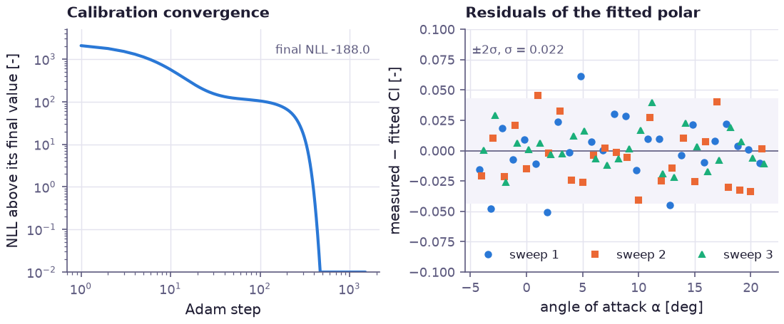
Left: the negative log-likelihood above its final value during the fit; after about 400 Adam steps it no longer changes. Right: the residuals of the 78 measurements, with the fitted scatter (σ = 0.022) as the ±2σ band. They show no trend with the angle of attack, also not through the stall, so the four-parameter curve captures the airfoil’s behaviour.

Step 3 — Turbulence and the approach as random inputs

Vertical gusts are a first-order Markov (Dryden-type) field with a scale length of 150 m, frozen in the air and flown through, sampled every 10 m. The field has unit variance; its intensity of the day is a separate random variable, as are the aircraft’s mass and the pilot’s speed keeping:

gust_shape = prp.RandomVariable(
    "gust",
    prp.ornstein_uhlenbeck(
        init=0.0, mean=0.0, theta=1.0 / GUST_SCALE, sigma=np.sqrt(2.0 / GUST_SCALE), n_steps=N_PATH, dt=DS
    ),
)
# RMS vertical gust velocity: light to moderate low-level turbulence.
gust_rms = prp.RandomVariable("gust_rms", prp.LogNormal(mu=np.log(1.1), sigma=0.45))  # [m/s]
mass = prp.RandomVariable("mass", prp.Uniform(900.0, MTOW))  # [kg]
speed_error = prp.RandomVariable("speed_error", prp.Gaussian(0.0, 1.0))  # pilot speed keeping [m/s]
target_speed = prp.Param("target_speed", init=APPROACH_SPEED)  # [m/s], a design variable

The response is quasi-steady: the aircraft is trimmed to carry its weight, and a vertical gust w adds atan(w / V) to the angle of attack. Over the 3 km of the approach this gives the worst margin to the stall angle and the peak load factor:

alpha_trim = _trim_alpha(weight / q_area, slope, a0, a_half, width)
w = rms[..., None] * z[..., N_SPINUP:]  # (..., 300) vertical gust [m/s]
alpha = alpha_trim[..., None] + jnp.rad2deg(jnp.arctan(w / v[..., None]))
load = q_area[..., None] * _wing_cl(alpha, slope, a0, a_half, width) / weight[..., None]
margin = _stall_angle(slope, a0, a_half, width) - jnp.max(alpha, axis=-1)

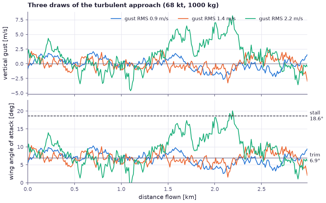
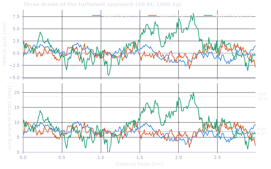
Three draws of the approach at 68 kt and 1000 kg. Top: the vertical gust along the flight path. Bottom: the wing’s angle of attack around its trim value of 6.9°. In the most turbulent draw (gust RMS 2.2 m/s) an updraft of about 7.5 m/s held for several hundred metres carries the wing past its stall angle of 18.6°; the shaded excursion is the stall.

Step 4 — Stall probability and the flight envelope

Both results are uncertain attributes of the same model as the tunnel data, so they use the calibrated parameters directly. The probability of stall is the cumulative distribution of the stall margin at zero, averaged over the random inputs by cdf(); changing the target_speed parameter moves the aircraft across the envelope:

p_stall = float(compiled.cdf("stall_margin", 0.0, params=raw))

pv = {**raw, "target_speed": jnp.asarray(v)}
ps = float(compiled.cdf("stall_margin", 0.0, params=pv))
pn = 1.0 - float(compiled.cdf("peak_load_factor", LIMIT_LOAD, params=pv))

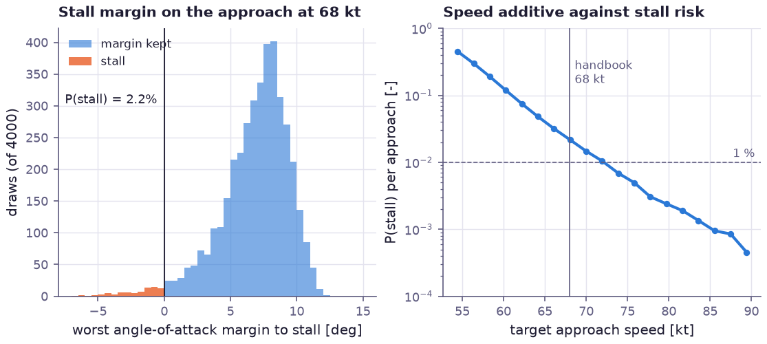
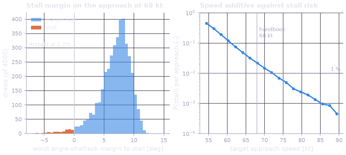
Left: the worst angle-of-attack margin on the approach at 68 kt. Most approaches keep 5 to 10° of margin; the draws below zero, 2.2 %, stall. Right: the probability of stall against the target approach speed. Each knot added to the handbook speed cuts the risk by roughly a sixth: a 4 kt gust additive brings it to 1 %, 6 kt to 0.7 %.

Step 5 — Sensitivities

local_sensitivity() differentiates the probability of stall with respect to the approach speed and the four calibrated lift-curve parameters, through the trim solution, the stall-angle solver and the Monte Carlo average. sobol_sensitivity() splits the variance of the stall margin among the random inputs:

local = prp.local_sensitivity(
    compiled, "stall_margin", "cdf", level=0.0, wrt=["target_speed", *AERO_NAMES], params=raw
)
sobol = prp.sobol_sensitivity(compiled, "stall_margin", n_samples=4096, params=raw)

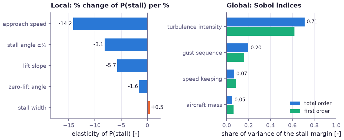
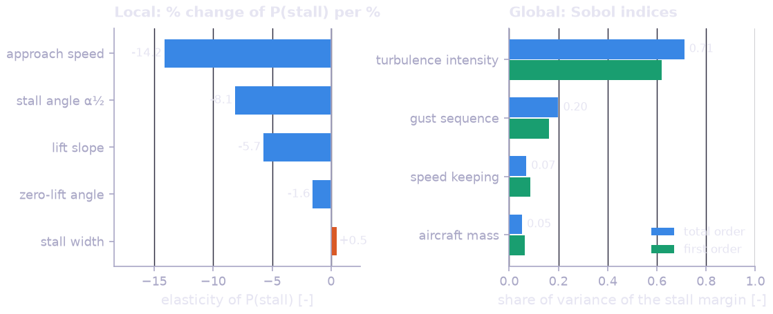
Left: elasticities of the stall probability. A 1 % faster approach lowers it by 14 %, a 1 % later separation (α½) by 8 %: the risk lives in the tail of the margin distribution, so small shifts of the margin change it a lot. The calibration pins these parameters to a fraction of a percent (see the output below), so the lift curve contributes little uncertainty to the answer. Right: Sobol indices of the stall margin. The day’s turbulence intensity explains 71 % of its variance and the particular gust sequence 20 %; mass and speed keeping matter little. The operational lever is therefore the speed additive in turbulence, not the loading of the aircraft.

Results

Output of python examples/airfoil_loads/model.py (about 12 s on a laptop CPU):

=== Calibration of the lift polar to three tunnel sweeps ===
ParameterUncertainty:
  fitted on 78 observations, log-likelihood 188.041
  alpha_half_deg = 15.5189 +/- 0.036  [15.4483, 15.5895]
  alpha_zero_deg = -2.96251 +/- 0.04706  [-3.05474, -2.87028]
  lift_slope = 6.23842 +/- 0.03236  [6.17499, 6.30185]
  stall_width_deg = 0.973593 +/- 0.01717  [0.939939, 1.00725]
  tunnel_noise = 0.0217158 +/- 0.001738  [0.0183085, 0.0251231]
  section Cl_max 1.599 at 13.5 deg; wing CL_max 1.599 at 18.6 deg
  stall speed at MTOW 26.2 m/s (51 kt); approach at 1.34 V_S
  wing CL_max 95 % interval [1.589, 1.610]

=== Stall risk on a 3 km turbulent final approach at 68 kt ===
  mean worst-case margin 6.9 deg, 1 % quantile -1.8 deg
  P(stall) = 2.19%   99 % peak load factor 2.03

=== Flight envelope: stall and limit-load exceedance vs airspeed ===
   28.0 m/s ( 54 kt): P(stall)  45.13%   P(n > 3.8)  0.000%
   31.0 m/s ( 60 kt): P(stall)  11.90%   P(n > 3.8)  0.000%
   35.0 m/s ( 68 kt): P(stall)   2.19%   P(n > 3.8)  0.000%
   38.0 m/s ( 74 kt): P(stall)   0.69%   P(n > 3.8)  0.000%
   42.0 m/s ( 82 kt): P(stall)   0.19%   P(n > 3.8)  0.000%
   50.0 m/s ( 97 kt): P(stall)   0.01%   P(n > 3.8)  0.060%
   60.0 m/s (117 kt): P(stall)   0.00%   P(n > 3.8)  0.316%
   70.0 m/s (136 kt): P(stall)   0.00%   P(n > 3.8)  0.900%
   80.0 m/s (156 kt): P(stall)   0.00%   P(n > 3.8)  1.642%

=== Local sensitivity of P(stall) at 68 kt ===
LocalSensitivity:
  cdf[stall_margin] = 0.0218669
  d/d target_speed = -0.008847  (elasticity -14.152)
  d/d alpha_half_deg = -0.01147  (elasticity -8.140)
  d/d lift_slope = -0.02014  (elasticity -5.744)
  d/d alpha_zero_deg = +0.01147  (elasticity -1.554)
  d/d stall_width_deg = +0.01091  (elasticity +0.486)

=== What drives the worst-case stall margin (Sobol) ===
SobolSensitivity:
  variance of stall_margin over 4096 samples
  gust_rms: first 0.620, total 0.711 (interaction +0.091)
  gust: first 0.162, total 0.199 (interaction +0.037)
  speed_error: first 0.087, total 0.070 (interaction -0.017)
  mass: first 0.065, total 0.052 (interaction -0.012)
  unexplained by first-order effects: 0.066

The probabilities are per approach through 3 km of turbulence whose intensity is drawn from the distribution above, not per flight hour; they compare speeds and configurations, and would be scaled by the exposure to turbulence for a risk budget.

Primitives exercised

Category	Used for
Param, op()	The lift-curve unknowns; the polar, lifting-line wing, stall-angle and trim solvers as graph nodes
calibrate(), parameter_uncertainty(), propagate(), sample_parameters()	Fit to the tunnel sweeps, standard errors, the interval of CL,max, the posterior bands
ornstein_uhlenbeck(), RandomVariable	The gust field along the flight path; turbulence intensity, mass and speed keeping
cdf(), quantile()	Probability of stall and of exceeding the limit load; load-factor quantiles across the envelope
local_sensitivity(), sobol_sensitivity()	Elasticities of the stall probability; attribution of the stall-margin variance

Running it

$ python examples/airfoil_loads/model.py