Example: Operational Fatigue Answers for a Wind Turbine

A wind farm operator decides every ten minutes whether a turbine may run at full power. The rule: derate when the 95 percent quantile of the tower base damage-equivalent load (DEL) over the next 30 minutes exceeds the design value of 10.5 MN m. The DEL comes from a prophys model. A turbulent wind series drives the rotor thrust, the thrust gives the tower base bending moment, and rainflow counting of that moment gives the load. One answer is a Monte Carlo run of 4096 wind series of 1800 steps each, about 90 ms, and the question returns for every turbine every ten minutes.

This chapter amortizes that answer with prophys.amortize(). It checks first that doing so pays off, validates the surrogate against the full model, and runs a whole day of operational queries through the guarded surrogate. The full runnable source is examples/operational_surrogate/model.py; it runs on the free tier in about five minutes on a laptop.

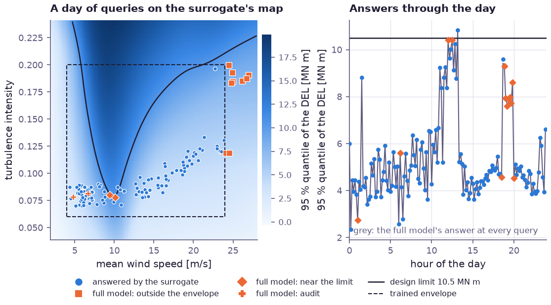
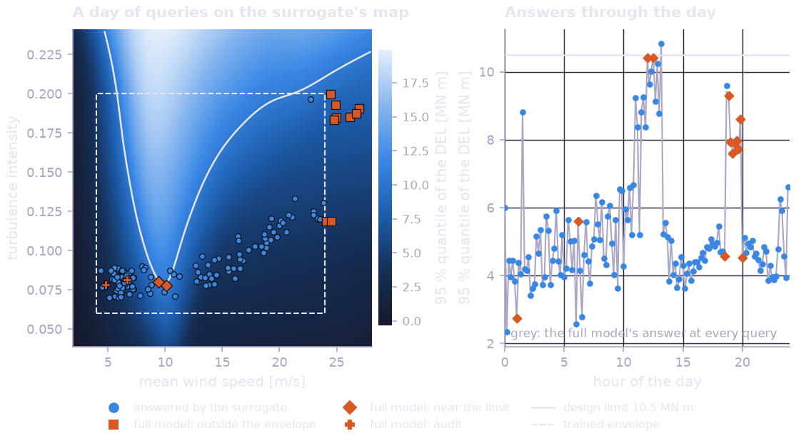
Left: the surrogate’s 95 percent quantile of the DEL over mean wind speed and turbulence intensity. The black line is the design limit and the dashed box the envelope the surrogate was trained on. The dots are the 144 ten-minute forecasts of one day: blue ones were answered by the surrogate, orange ones by the full model, with the marker giving the reason. Right: the answers through the day against the full model’s answer at every query (grey). 131 of the 144 queries were answered by the surrogate, in 0.29 ms each (median). 13 went to the full model: the evening storm left the envelope, where the ensemble members also disagree; two queries were within the tolerated error of the limit; and three were random audits. Every derating decision equals the one the full model alone would have taken.

Step 1 — The full model

The mean wind speed and the turbulence intensity are the operational inputs, so they are declared as Param leaves. The wind over 30 minutes is an Ornstein-Uhlenbeck process around the mean, with an integral time scale of 20 s. Below rated wind the thrust coefficient is constant; above it the blades pitch and the thrust falls. Rainflow counting of the tower base moment with a Wohler exponent of 4 gives the 1 Hz damage-equivalent load, with a 5 percent log-normal uncertainty for the rest of the load chain:

wind_speed = prp.Param("wind_speed", init=12.0, bounds=(3.0, 30.0))  # 10 minute mean [m/s]
turbulence = prp.Param("turbulence", init=0.12, bounds=(0.02, 0.4))  # intensity sigma_u / U

theta = 1.0 / TAU
wind = prp.RandomVariable(
    "wind",
    processes.ornstein_uhlenbeck(
        wind_speed, wind_speed, theta, turbulence * wind_speed * np.sqrt(2.0 * theta), T_STEPS, DT
    ),
)
v = prp.clip(wind, 0.0, 40.0)
ct = prp.where(v < RATED, CT_BELOW, CT_BELOW * (RATED / prp.maximum(v, RATED)) ** 2.5)
thrust = 0.5 * RHO * np.pi * ROTOR_RADIUS**2 * ct * v**2 / 1e6  # [MN]
moment = thrust * HUB_HEIGHT  # tower base bending moment [MN m]
damage = physics.fatigue_damage(moment, sn_exponent=WOHLER, sn_coefficient=1.0)
del_expr = (damage / T_STEPS) ** (1.0 / WOHLER)  # 1 Hz damage-equivalent load [MN m]
# model and measurement uncertainty of the load chain, 5 percent
tower_del = prp.UncertainAttribute("del", prp.LogNormal(prp.log(del_expr), 0.05), unit="MN*m")
model = prp.ProbabilityModel(tower_del)

A full operational answer is model.compile(n_samples=4096) followed by the statistics of 4096 draws. The Monte Carlo error of that answer is the yardstick for everything below.

Step 2 — Does amortizing pay off?

prophys.break_even() times one full answer, a batch of design points, a few training steps and one surrogate query, before anything is trained:

est = prp.break_even(
    model, "del", ENVELOPE, n_samples=N_OP, n_points=n_points, n_draws=n_draws, n_steps=n_steps, queries=144 * 365
)

BreakEvenEstimate:
  full_query_seconds = 0.081773
  surrogate_query_seconds = 0.0002563
  fallback_rate = 0.05
  data_seconds = 22.6552
  train_seconds = 85.1523
  effective_query_seconds = 0.00434498
  speedup = 18.8201
  break_even_queries = 1392.36
  queries = 52560
  pays_off = True
  recommendation = pays off after 1.39e+03 queries at a 18.8x speedup (expected queries exceed it)

With the assumed 5 percent of fallbacks, the up-front cost is recovered after about 1400 queries: ten days of one turbine’s queries, or one day of a ten-turbine farm’s. The training-time estimate is extrapolated from a few steps and came out low (85 s against the 224 s measured in Step 3); the measured costs give the final verdict in Step 5. A model that answered in a millisecond would not be worth amortizing at all.

Step 3 — Amortize and check the acceptance card

op = prp.amortize(
    model,
    "del",
    ENVELOPE,
    n_points=n_points,
    n_draws=n_draws,
    n_samples=N_OP,
    stats=STATS,
    thresholds={"quantile:0.95": DEL_LIMIT},
    n_steps=n_steps,
    n_validation=32,
    reference_draws=8 * N_OP,
    members=3,
    seed=0,
)

The full model runs at 4000 Latin hypercube points of the envelope, 256 wind series each, in vectorised batches. A location and scale network and an ensemble of three histogram-head networks learn the distribution of the DEL over the envelope. They are validated at 32 fresh points against reference runs with 32 768 series each:

AmortizationCard:
  attribute del, 4000 points x 256 draws, yardstick 4096 full-model draws
  statistic          surrogate  Monte Carlo      N_eq  ok
  quantile:0.95        0.02876      0.03818  7.22e+03  yes
  prob:>10.5          0.001607     0.001667  4.41e+03  yes
  CRPS 0.3788 (floor 0.3785), coverage {'50': 0.503, '90': 0.901, '98': 0.979}
  full query 89.6 ms, surrogate query 0.312 ms, data 26.5 s, training 224 s

Averaged over the envelope, both served statistics beat the full model’s own Monte Carlo error at 4096 draws: the surrogate is worth 7200 and 4400 full-model draws. Its CRPS is within 0.1 percent of the best reachable one.

The average hides where the errors are. Along a transect at turbulence intensity 0.12, which crosses the sharp load peak at rated wind, the same surrogate is worth only about 2200 draws for the 95 percent quantile, and 900 to 1100 for the median, the 99 percent quantile and the CVaR (right panel below). This operator serves only the two decision statistics, and the threshold gate sends every query whose 95 percent quantile is close to the limit back to the full model. At the peak itself the quantile is far above the limit, so the decision there is not in doubt. A stricter operator would add points near rated wind, or accept the card only per region.

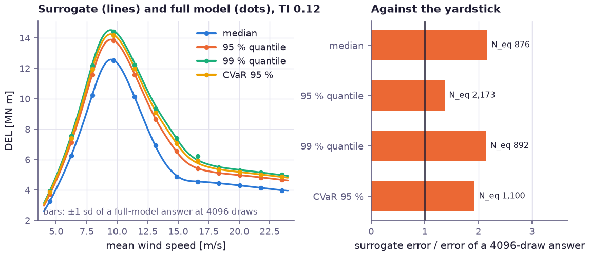
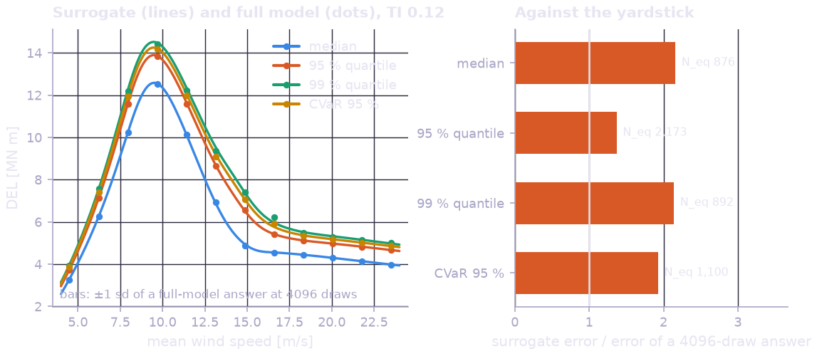
Left: along a transect at turbulence intensity 0.12, the surrogate’s statistics (lines) against ground truth from 65 536 full-model draws per point (dots). The bars are plus and minus one standard deviation of a 4096-draw full-model answer. The kink at rated wind (11.5 m/s), where the pitch control cuts the thrust, is learned. Right: on the transect, the surrogate’s error divided by the error of a 4096-draw full-model answer, and the equivalent number of full-model draws. On this transect every statistic is above one, less accurate than a 4096-draw answer. The errors concentrate around the peak at rated wind; the envelope-wide validation of the card averages them with the easier regions.

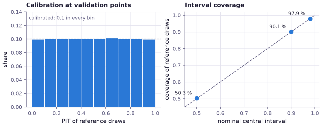
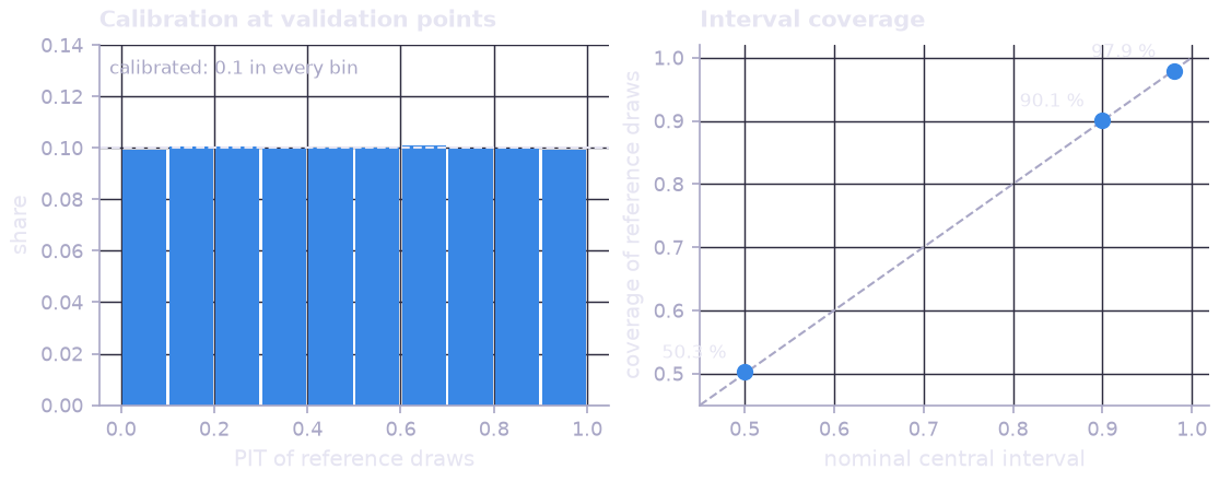
Calibration on the card’s validation points: the PIT histogram of the reference draws under the surrogate’s predictive distribution is flat, and the central 50, 90 and 98 percent intervals cover 50.3, 90.1 and 97.9 percent of the reference draws.

Step 4 — One operational day

The day brings a front: a calm morning, rising wind through rated in the afternoon, and a gusty storm peak in the evening that goes beyond the trained envelope. Each ten-minute forecast is one query:

ans = op.answer({"wind_speed": u, "turbulence": ti})

day: 131 answers from the surrogate (0.29 ms median), 13 from the full model (89 ms median)
fallbacks by reason: {'outside_support': 9, 'disagreement': 7, 'near_threshold': 2, 'audit': 3}
derating decisions equal to the full model's: 100 percent
pays off after 3.09e+03 queries at a 10.7x speedup (expected queries exceed it)

A query can have several reasons: the storm queries outside the envelope were mostly flagged by member disagreement too. Every query outside the envelope, and every query whose 95 percent quantile was within the tolerated error of the limit, went to the full model; op.log holds each of them with its reason and both answers. Because the queries near the limit are the ones the full model answers, every derating decision of the day equals the one the full model alone would have taken.

Step 5 — Speedup against fallback rate

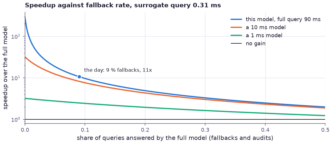
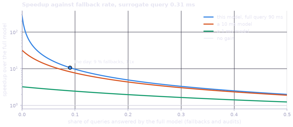
The expected speedup of the guarded surrogate over the full model, against the share of queries that fall back (fallbacks plus the one percent of audits), for this model and for hypothetical models whose full answer takes 10 ms and 1 ms. With a surrogate query of 0.31 ms, a 1 ms model gains at best a few times, and fallbacks erase even that. This model’s day, with 9 percent fallbacks, ran 11 times faster than the full model alone.

With the measured costs and the day’s 9 percent of fallbacks, amortizing pays off after about 3100 queries at an 11x speedup. The speedup is c_full / (c_surrogate + r c_full) for a fallback rate r. It is bounded by 1 / r however cheap the surrogate is, which is why the guard is tuned to send back only the queries that matter. Amortizing pays when the full answer is expensive (about 100 ms or more) and the queries are many; see Operational surrogates.

Running it

$ python examples/operational_surrogate/model.py

The figures come from docs/generate_example_operational_surrogate.py, which runs the example and adds the ground-truth transect.