

Example: Wind Farm Yield with Blade Element Momentum#
A developer must state the annual energy production (AEP) of a planned
16-turbine offshore farm together with the exceedance levels a lender asks
for, P50 and P90, and wants to know whether rearranging the turbines inside
the lease area recovers some of the energy lost to wakes. This chapter builds
the whole chain in one differentiable model: a blade element momentum (BEM)
rotor model wrapped as a symbolic operation, gradient ascent on its power
coefficient, a wind climate fitted to a year of met-mast records and held as a
DirectionalMixture, Gaussian wakes swept through
the farm with directional_sweep(), the uncertain inputs
of a yield assessment as RandomVariable leaves, the
AEP distribution with its quantiles, a Sobol decomposition of the yield
uncertainty, and a gradient-based layout optimisation. The full runnable
source is examples/wind_farm/model.py.
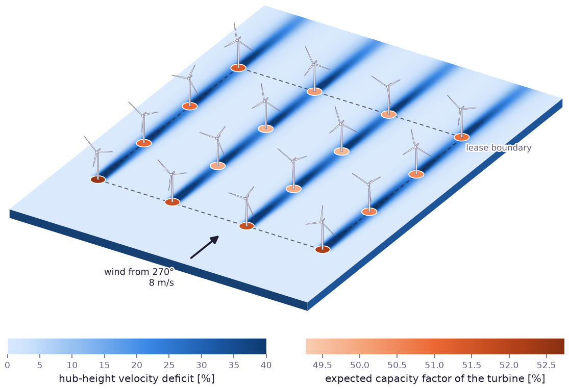
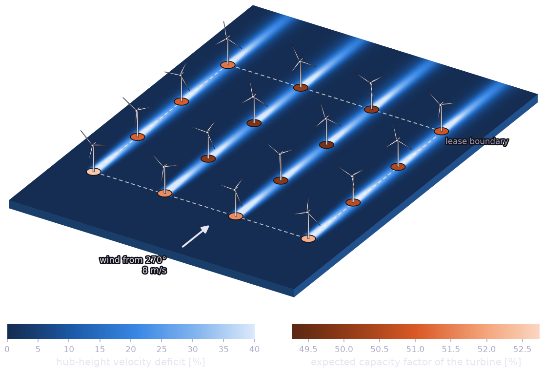
The optimised farm in the prevailing westerly at 8 m/s, seen from the south-west. The sea surface is coloured by the hub-height velocity deficit computed with the same directional sweep as the yield model: every wake widens downstream and the second and later turbines of a row sit in the wakes of those ahead. Each foundation is coloured by the turbine’s expected capacity factor over the whole wind climate; the turbines on the western edge, upwind in the prevailing winds, yield most. Turbines are drawn at 2.8 times their size.
Step 1 — Airfoil and blade#
The rotor has three 65 m blades. Their airfoil is described by a smooth polar:
thin-airfoil lift slope, trailing-edge stall by Kirchhoff’s flow model with the
separation point of Leishman and Beddoes, and a drag that blends into
flat-plate drag as the flow separates. A drag_factor scales the
attached-flow drag and later represents leading-edge erosion:
def airfoil_polar(alpha, drag_factor=1.0):
    """Lift and drag coefficients at angle of attack `alpha` [rad]. The
    attached-flow drag (profile drag plus a lift-dependent term, maximum
    lift-to-drag ratio ~80) is scaled by `drag_factor` to represent
    leading-edge erosion, and blends into flat-plate drag as the flow
    separates."""
    f = separation_point(alpha)
    cl_attached = LIFT_SLOPE * (alpha - ALPHA_ZERO_LIFT)
    cl = cl_attached * ((1.0 + jnp.sqrt(f)) / 2.0) ** 2
    cd_attached = drag_factor * (0.008 + 0.006 * (cl_attached - 0.4) ** 2)
    cd = f * cd_attached + (1.0 - f) * (0.02 + 1.9 * jnp.sin(alpha) ** 2)
    return cl, cd
The chord and twist follow the optimum blade shape for a design tip speed ratio of 8 (Manwell et al., with wake rotation), the root chord capped at 4.6 m.
Step 2 — BEM theory as a symbolic operation#
Each of 30 blade elements balances the momentum removed from its annulus
against the blade forces. One update of the axial induction a and the
tangential induction a' uses the inflow angle from the velocity triangle,
Prandtl’s tip loss F and Buhl’s high-induction correction; a fixed number
of under-relaxed iterations makes the solver a finite, differentiable
computation:
def step(_, state):
    a, ap = state
    phi, _, cn, ct = loads(a, ap)
    sin_phi = jnp.maximum(jnp.abs(jnp.sin(phi)), 1e-4)
    tip = jnp.exp(-N_BLADES * (R - r_el) / (2.0 * r_el * sin_phi))
    F = jnp.maximum(2.0 / jnp.pi * jnp.arccos(jnp.clip(tip, 0.0, 1.0 - 1e-7)), 1e-3)
    a_momentum = 1.0 / (4.0 * F * jnp.sin(phi) ** 2 / (solidity * cn) + 1.0)
    ct_local = solidity * (1.0 - a) ** 2 * cn / sin_phi**2
    disc = jnp.maximum(ct_local * (50.0 - 36.0 * F) + 12.0 * F * (3.0 * F - 4.0), 1e-9)
    a_buhl = (18.0 * F - 20.0 - 3.0 * jnp.sqrt(disc)) / (36.0 * F - 50.0)
    a_new = jnp.where(ct_local > 0.96 * F, a_buhl, a_momentum)
    ap_new = jnp.clip(1.0 / (4.0 * F * jnp.sin(phi) * jnp.cos(phi) / (solidity * ct) - 1.0), -0.5, 0.5)
    return 0.7 * a + 0.3 * a_new, 0.7 * ap + 0.3 * ap_new  # under-relaxed update

a, ap = jax.lax.fori_loop(0, BEM_ITERATIONS, step, (jnp.full(shape, 0.3), jnp.zeros(shape)))
The power coefficient integrates the tangential blade force over the span.
op() wraps the JAX solver as a node of the symbolic
graph, so Cp accepts constants, parameters or random variables:
def power_coefficient(tsr, pitch_deg, drag_factor=1.0) -> prp.Expr:
    """``Cp(tsr, pitch)`` of the rotor as a symbolic expression."""
    return op("bem_cp", lambda lam, b, d: _bem(lam, b, d)[0], tsr, pitch_deg, drag_factor)
Step 3 — The optimal operating point#
With the tip speed ratio and the blade pitch as Param
leaves, optimize() climbs the Cp surface by gradient
ascent; the gradients pass through all 100 BEM iterations:
tsr_param = prp.Param("tip_speed_ratio", init=7.0)
pitch_param = prp.Param("pitch_deg", init=0.0)
rotor_cp = power_coefficient(tsr_param, pitch_param)


def optimise_operating_point(n_steps: int = 150):
    return prp.optimize(-rotor_cp, wrt=[tsr_param, pitch_param], n_steps=n_steps, learning_rate=0.1)
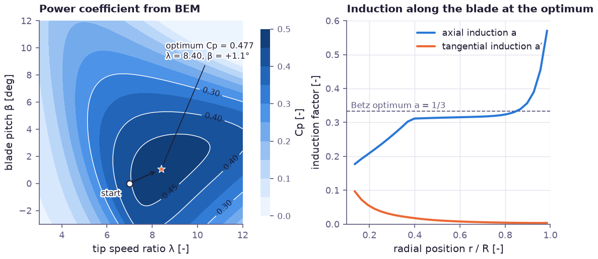
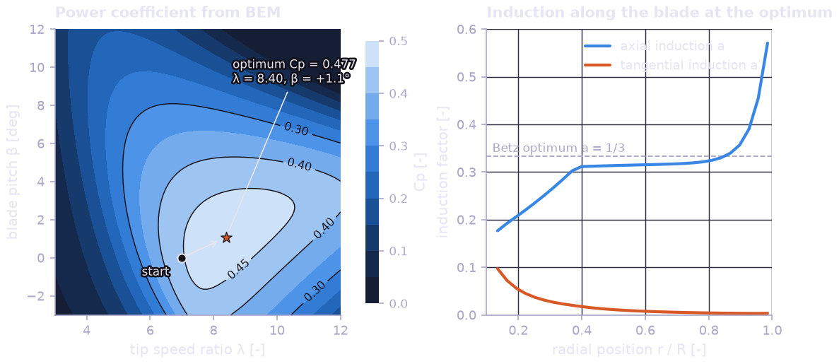
Left: the power coefficient over tip speed ratio and pitch, with the start and the end of the gradient ascent. The optimum, Cp = 0.477 at a tip speed ratio of 8.4 and 1.1° of pitch, lies on a broad ridge, which is why a variable-speed rotor loses little when it cannot hold the optimum exactly. Right: the induction along the blade at that optimum. The axial induction sits just below the Betz value 1/3 over the outer blade, where most power is produced, and rises at the tip where the tip loss concentrates the loading; the tangential induction (wake rotation) matters only near the root.
Step 4 — Power curve with uncertainty#
The turbine runs at the optimal tip speed ratio until its tip speed reaches
85 m/s, and pitches above rated power (4.5 MW) to hold it. The power curve of
the turbine as built is uncertain: air density varies with the season and
leading-edge erosion raises the blade drag. Both are random variables that
enter the BEM operation directly, and the curve on a grid of wind speeds is a
path-valued UncertainAttribute:
air_density = prp.RandomVariable("air_density", prp.Gaussian(AIR_DENSITY, 0.025))
drag_factor = prp.RandomVariable("drag_factor", prp.LogNormal(mu=0.0, sigma=0.35))

curve = electrical_power(
    jnp.asarray(SPEED_GRID), tsr_opt, partial_load_pitch, column(air_density), column(drag_factor)
)
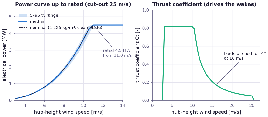
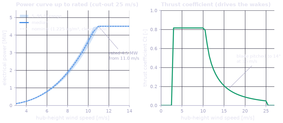
Left: the power curve up to rated, the median and the 5–95 % range over air density and blade erosion. The spread is widest just below rated speed, where the turbine produces a large share of its energy and every percent of Cp shows in the yield. Right: the thrust coefficient that sets the strength of the wakes. It stays near 0.8 below rated and falls quickly once the blades pitch, so wake losses matter most at moderate wind speeds.
Step 5 — The wind climate from a met mast#
A year of hourly records (direction and speed at hub height) is split into
twelve 30° sectors. fit_distribution() fits a Weibull
distribution to each sector by maximum likelihood; the sector frequencies and
fits assemble into one directional climatology:
for k in range(N_SECTORS):
    weibull = prp.Weibull(
        scale=prp.Param(f"scale_{k}", init=9.0, transform="softplus"),
        concentration=prp.Param(f"shape_{k}", init=2.0, transform="softplus"),
    )
    fit = prp.fit_distribution(weibull, record[sector == k, 1], n_steps=n_steps, learning_rate=0.1)
    fits.append(fit)
    speeds.append(prp.Weibull(scale=float(fit.params[f"scale_{k}"]), concentration=float(fit.params[f"shape_{k}"])))
frequency = np.bincount(sector, minlength=N_SECTORS) / len(sector)
climate = prp.DirectionalMixture.evenly_spaced(weights=frequency, intensities=speeds)
The farm is evaluated on a table of 72 directions by 30 speed bins, each
weighted by the climatology’s joint density climate.log_prob(direction,
intensity).
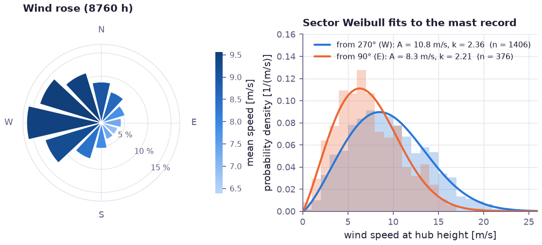
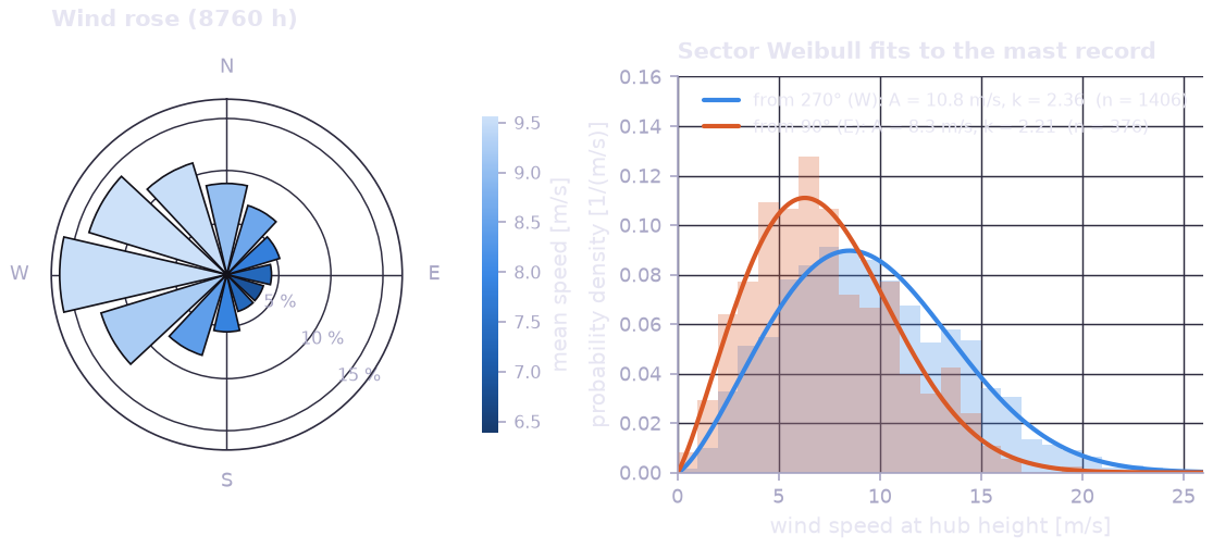
Left: the wind rose of the mast year, bars coloured by the sector’s mean wind speed; westerlies are both the most frequent and the strongest winds. Right: the Weibull fits of the westerly and the easterly sector against the records they were fitted to. The easterly winds are rarer and weaker, so the wakes of the prevailing direction dominate the losses.
Step 6 — Wakes swept through the farm#
For every flow case the turbines are processed from upwind to downwind. Each
turbine’s inflow is the free stream reduced by the Gaussian deficits of the
turbines upstream of it (Bastankhah and Porté-Agel), each scaled by that
upstream turbine’s own local speed and combined as a root sum of squares. The
deficit, linearised in the far wake, maps onto the kernel of
directional_sweep():
def wake_parameters(ct):
    """Gaussian wake of Bastankhah & Porte-Agel (2014), linearised in the
    far wake: deficit ``Ct / (16 (sigma/D)^2)`` with ``sigma = k x + eps D``,
    ``eps = 0.2 sqrt(beta)``, ``beta = (1 + sqrt(1 - Ct)) / (2 sqrt(1 - Ct))``.
    In the kernel of `directional_sweep` this is ``width = eps D`` and
    ``strength = Ct / (16 eps^2)``; returns ``(strength, width)``."""
    root = prp.sqrt(prp.clip(1.0 - ct, 0.05, 1.0))
    eps = 0.2 * prp.sqrt(0.5 * (1.0 + root) / root)
    return ct / (16.0 * eps**2), eps * ROTOR_DIAMETER

local_speed = physics.directional_sweep(
    layout,
    _flat(inflow),
    direction=_flat(direction),
    strength=_flat(strength),
    width=_flat(width),
    growth=_flat(growth),
    combine="rss",
)  # (batch * C, T)
All 2160 flow cases (and, later, all Monte Carlo draws) go through one batched
call over the 16 turbine positions. The power of each turbine follows from the
power curve as a TableLookup1D, and its
expectation over the climate from the case probabilities.
Step 7 — The yield assessment: P50 and P90#
Four inputs of the assessment are uncertain: the long-term mean wind speed (the mast year and its long-term correction), the wake expansion rate, the power-curve performance of the delivered turbines, and the downtime:
# Long-term mean wind speed relative to the mast estimate (measurement and
# long-term correction uncertainty, 4 % on speed).
speed_factor = prp.RandomVariable("resource", prp.Gaussian(1.0, 0.04))
# Wake expansion rate k* for offshore turbulence intensities of 6-9 %.
wake_growth = prp.RandomVariable("wake_growth", prp.Uniform(0.022, 0.040))
# Power-curve performance relative to the BEM prediction (2 %).
performance = prp.RandomVariable("power_curve", prp.Gaussian(1.0, 0.02))
# Fraction of the year the turbines are down (median 3.5 %).
downtime = prp.RandomVariable("downtime", prp.LogNormal(mu=np.log(0.035), sigma=0.35))
The long-term AEP is a symbolic function of all four. The production of a single year scatters around it with the inter-annual variability of the wind (6 %); the mean over ten years scatters by that amount divided by the square root of ten:
availability = 1.0 - prp.clip(downtime, 0.0, 0.3)
aep_long_term = HOURS_PER_YEAR * performance * availability * prp.sum_(turbine_power, axis=-1) / 1e9  # [GWh]
aep_1y = prp.UncertainAttribute(
    "aep_1y",
    prp.Gaussian(aep_long_term, INTERANNUAL_VARIABILITY * aep_long_term),
    unit="GWh",
    domain="energy production of a single year",
)
P50 is the median and P90 the level exceeded with 90 % probability, the 10 % quantile, both read from the compiled model; the Sobol analysis splits the variance of the long-term AEP (relative to the central estimate) among the four inputs:
p50 = float(compiled.quantile("aep_1y", 0.5))
p90 = float(compiled.quantile("aep_1y", 0.1))
p90_10 = float(compiled.quantile("aep_10y", 0.1))

sobol = prp.sobol_sensitivity(results["optimised"]["compiled"], "aep_deviation", n_samples=1024)
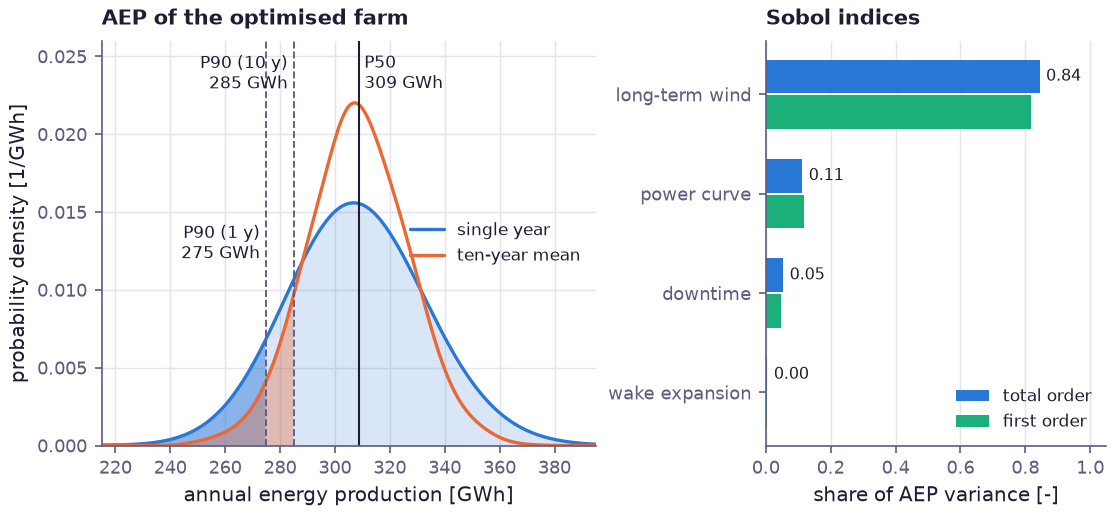
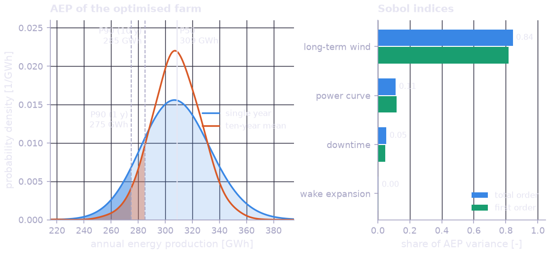
Left: the AEP of the optimised farm for a single year and as a ten-year mean, with the shaded tails below the respective P90. Averaging over ten years removes most of the weather’s year-to-year scatter, which lifts the P90 from 275 to 285 GWh; what remains is the uncertainty of the assessment itself. Right: the Sobol indices of that remaining uncertainty. The long-term wind resource carries 84 % of the variance, because power grows with a high power of the wind speed; wake expansion, though it sets the wake loss, contributes less than 1 %. Further measurement at the site pays off, more wake modelling does not.
Step 8 — Layout optimisation#
The turbine positions become a single (16, 2) parameter. The objective is
the expected farm power over the full climate; the lease boundary and a
minimum spacing of four rotor diameters are constraints, enforced as
penalties by optimize(). The gradient of the farm power
with respect to every coordinate comes from the directional sweep itself:
result = prp.optimize(
    -farm_mw,
    wrt=[layout],
    constraints=[outside, too_close],
    penalty_weight=1e4,
    n_steps=n_steps,
    learning_rate=learning_rate,
)
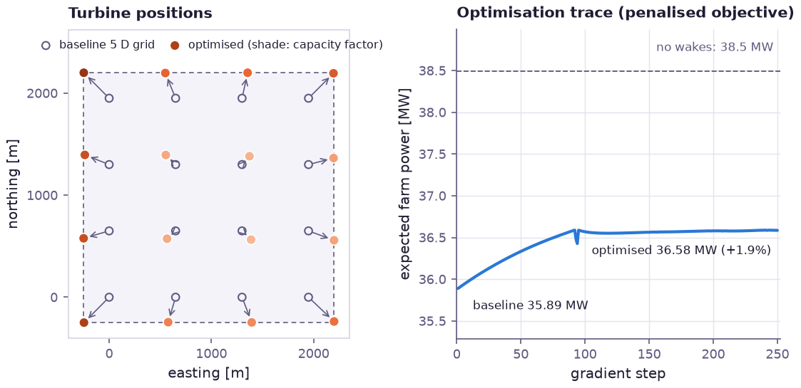
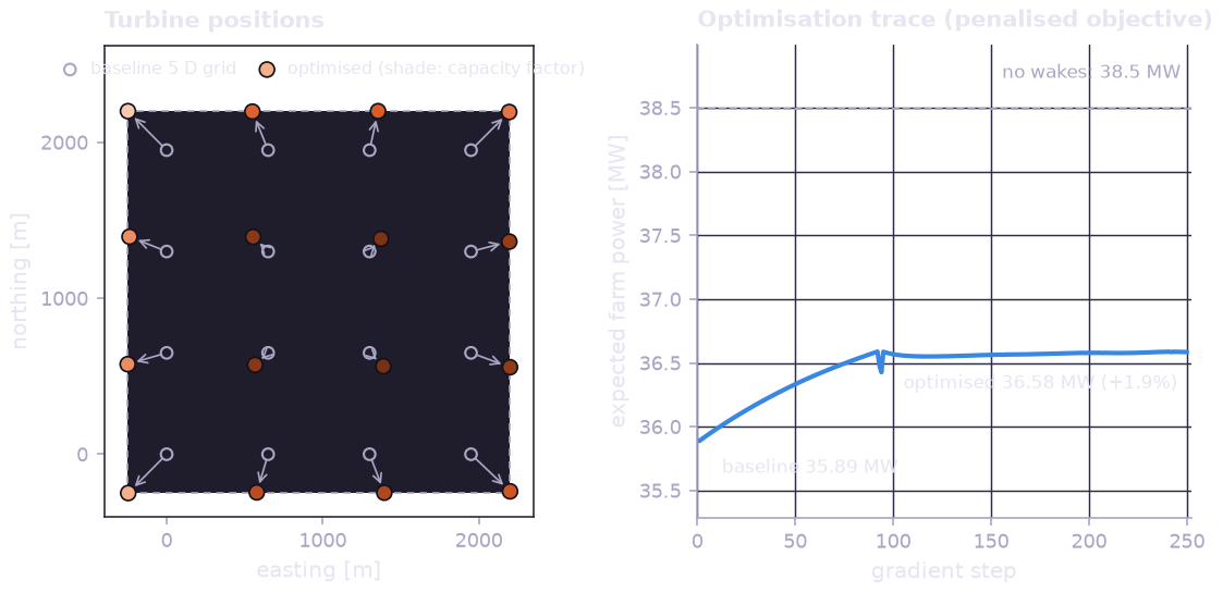
Left: the baseline 5 D grid (open circles) and the optimised positions, shaded by expected capacity factor. The optimiser spreads the farm to the lease boundary, which lengthens the spacing between turbines from 5 D to about 6.3 D in both directions; every turbine gains 0.3 to 1.4 points of capacity factor. Right: the expected farm power during the optimisation. It rises from 35.9 to 36.6 MW, +1.9 %, which cuts the wake loss from 6.8 % to 5.0 %; the brief dip is a step into the boundary penalty, which the next steps undo.
Results#
Output of python examples/wind_farm/model.py (about 40 s on a laptop CPU):
=== Rotor: optimal operating point (gradient ascent through BEM) ===
  Cp: 0.446 at (7.0, 0.0 deg) -> 0.477 at tip speed ratio 8.40, pitch +1.08 deg (Ct 0.82)
  rated power 4.5 MW reached at 11.0 m/s; pitch at 25 m/s 24.4 deg
  power at 9 m/s: 2.66 MW nominal, 10-90 % range [2.49, 2.78] MW (air density, blade erosion)

=== Wind climate (per-sector Weibull fits to 8760 hourly records) ===
  from   270 deg: 16.1%  A=10.76 m/s  k=2.36
  from   240 deg: 12.6%  A=10.43 m/s  k=2.22
  ...
  from   300 deg: 13.8%  A=10.80 m/s  k=2.36
  mean wind speed 8.85 m/s

=== Farm flow and wake losses (nominal inputs) ===
  gross (no wakes) 38.49 MW, baseline layout 35.89 MW, wake loss 6.8%
  capacity factor per turbine: 48.3% .. 52.2%

=== Layout optimisation (4 D minimum spacing, inside the lease) ===
  expected farm power 35.89 -> 36.58 MW (+1.9%), wake loss 5.0%
  closest pair 6.09 D, layout within [-250, 2200] m

=== Yield assessment: AEP distribution ===
  baseline : central 303.6  mean 302.5  P50 302.8  P90 (1 y) 269.1  P90 (10 y) 279.2 GWh
  optimised: central 309.5  mean 308.3  P50 308.7  P90 (1 y) 274.8  P90 (10 y) 284.9 GWh

=== What drives the yield uncertainty (Sobol, long-term AEP) ===
SobolSensitivity:
  variance of aep_deviation over 1024 samples
  resource: first 0.817, total 0.844 (interaction +0.027)
  power_curve: first 0.118, total 0.112 (interaction -0.006)
  downtime: first 0.046, total 0.053 (interaction +0.008)
  wake_growth: first 0.002, total 0.005 (interaction +0.003)
  unexplained by first-order effects: 0.017
The layout change is worth 5.9 GWh a year at P50 and 5.7 GWh at the ten-year P90. The P90 sits 11 % below the P50 for a single year and 8 % below it over ten years.
Primitives exercised#
Category |
Used for |
|---|---|
The BEM solver as a differentiable graph node; the optimal tip speed ratio and pitch; the layout |
|
Sector fits to the mast record and the directional climatology |
|
Wake shadowing for every flow case and every Monte Carlo draw in one batched call |
|
Power and thrust curves |
|
Air density and erosion (power curve); resource, wake expansion, performance and downtime (AEP) |
|
P50 / P90 and the attribution of the yield uncertainty |
Running it#
$ python examples/wind_farm/model.py