Example: Aggregate Losses and a Stop-Loss Layer

A commercial property insurer expects about 120 claims a year. Claim sizes are heavy tailed and paid up to a policy limit of EUR 2.5 million, and the number of claims varies more from year to year than a Poisson count would. The insurer holds capital against the worst 1 % of years and is offered an aggregate stop-loss treaty “15 xs A”: the reinsurer pays the part of the annual loss between the attachment A and A + 15 million, for a premium of 1.5 times the expected layer loss. The example calibrates the claim-size distribution to censored claims data, computes the exact aggregate loss distribution with compound_distribution() (Panjer’s recursion), prices the layer, differentiates premium and capital with respect to the treaty terms and the severity tail, chooses the attachment by gradient descent with optimize(), checks everything against Monte Carlo, and couples a second line of business through a GaussianCopula. All amounts are in EUR million. The full runnable source is examples/insurance_layers/model.py.

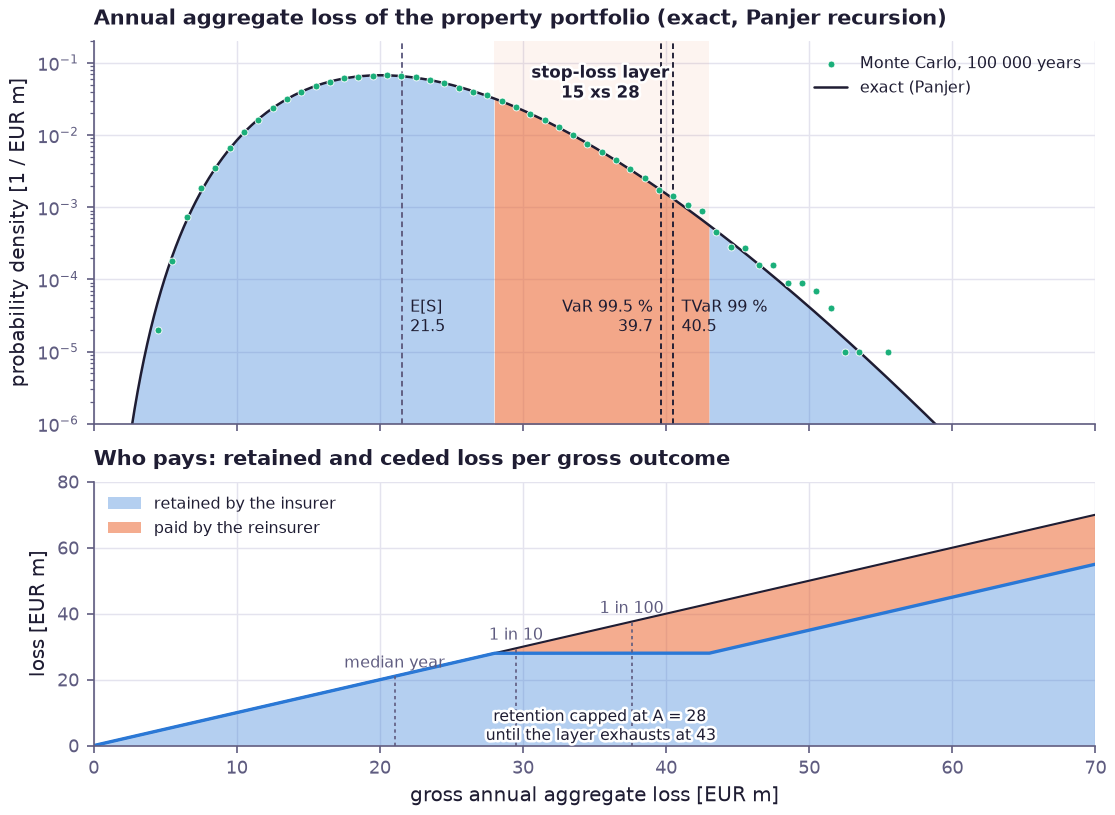
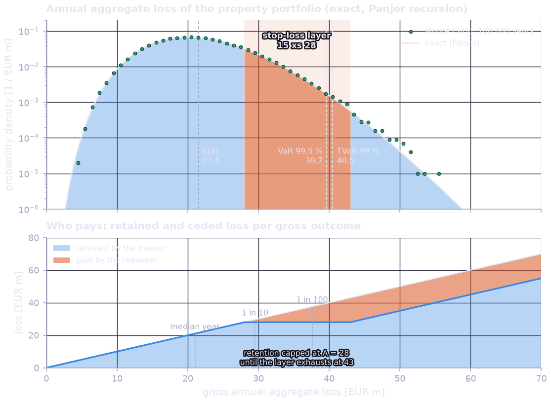
Top: probability density of the annual aggregate loss on a log scale, exact from Panjer’s recursion (line), with a histogram of 100 000 simulated years (dots) on top of it. The optimal layer, 15 xs 28, is shaded orange: it covers the losses between roughly the 1-in-7 and the 1-in-650 year level, and the 99.5 % value-at-risk and the 99 % tail value-at-risk both fall inside it. Bottom: how a gross annual loss splits between insurer and reinsurer. The insurer’s retained loss rises with the gross loss up to the attachment, stays flat across the layer and rises again once the layer is exhausted at 43 million.

Step 1 — Severity from censored claims

The claims record holds 600 paid amounts. Ten were paid at the policy limit, which says only that the loss was at least 2.5 million, so they enter the fit as right-censored observations. The claim size is a log-normal with learnable median and log-sd, fitted with calibrate():

log_median = prp.Param("mu", init=np.log(0.1))  # log of the median claim [log EUR m]
log_sd = prp.Param("sigma", init=1.0, transform="softplus")  # log-sd of the claim size
severity = prp.LogNormal(log_median, log_sd)

claim_size = prp.UncertainAttribute("claim_size", severity, unit="EUR m", domain="ground-up claim size")
claims_model = prp.ProbabilityModel(claim_size)

paid = claims_record()
at_limit = paid >= POLICY_LIMIT
observations = prp.Observations.right_censored(paid, censored=at_limit)
compiled = claims_model.compile()
fit = prp.calibrate(compiled, "claim_size", observations, n_steps=1000, learning_rate=0.05)

Step 2 — The exact aggregate distribution

The severity is discretised on a lattice of EUR 10 000 steps by the rounding method, with every loss above the policy limit paid at the limit. Because the discretisation uses the distribution’s own cdf, the lattice pmf is a differentiable function of mu and sigma. The claim count is negative binomial with mean 120 and variance 600, a Poisson count whose rate itself varies from year to year. compound_distribution() then returns the pmf of the annual total on 8 000 lattice points:

def severity_lattice(dist) -> prp.Expr:
    edges = (np.arange(1, N_SEVERITY) - 0.5) * STEP
    cdf = dist.cdf(jnp.asarray(edges))
    return op(
        "rounding_pmf",
        lambda c: jnp.diff(jnp.concatenate([jnp.zeros(1), c, jnp.ones(1)])),
        cdf,
    )


severity_pmf = severity_lattice(severity)
aggregate_pmf = physics.compound_distribution(
    severity_pmf,
    family="negative_binomial",
    shape=COUNT_SHAPE,
    probability=COUNT_SCALE,
    n_out=N_AGGREGATE,
)  # P(S = k STEP), exact for the lattice severity

Panjer’s recursion is exact for the lattice severity: there is no sampling error, and the tail beyond the 1-in-1000 year level is as accurate as the body. Tail measures are sums over the pmf. The tail value-at-risk weights the lattice cell at the quantile fractionally, so it is continuous in every argument:

def tail_value_at_risk(values, pmf, alpha: float) -> prp.Expr:
    tail_weight = op(
        "tail_weight",
        lambda p: jnp.clip(jnp.cumsum(p) - alpha, 0.0, p),
        pmf,
    )
    return prp.sum_(values * tail_weight) / (1.0 - alpha)

Step 3 — Price, capital and their gradients

The layer loss is the gross loss above the attachment, capped at the limit. The premium is 1.5 times its expectation. The capital is the 99 % tail value-at-risk of the retained loss in excess of its mean, and the total annual cost of the programme is the reinsurer’s margin plus 10 % cost of capital:

attachment = prp.Param("attachment", init=20.0)  # A [EUR m]
limit = prp.Param("limit", init=15.0)  # L [EUR m]

s = jnp.asarray(AGGREGATE)
ceded = prp.minimum(prp.relu(s - attachment), limit)  # layer loss per lattice value
net = s - ceded  # retained, non-decreasing in s

expected_layer_loss = expected(ceded, aggregate_pmf)
premium = (1.0 + LOADING) * expected_layer_loss
capital = tail_value_at_risk(net, aggregate_pmf, ALPHA) - expected(net, aggregate_pmf)
total_cost = premium - expected_layer_loss + COST_OF_CAPITAL * capital

premium and capital are expressions of the treaty terms and of the severity parameters (through the compound pmf), so jax.grad of expr.evaluate(env) gives exact sensitivities to all of them in one pass. The optimal attachment follows from the same expression:

opt = prp.optimize(total_cost, wrt=[attachment], n_steps=400, learning_rate=0.1, extra_env=dict(env, limit=15.0))

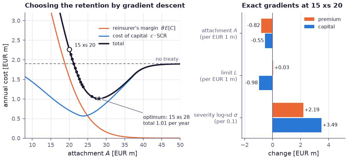
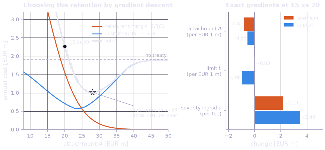
Left: the reinsurer’s margin falls and the cost of capital rises as the attachment moves up; their sum, the total cost, has a clear minimum. The offered 15 xs 20 costs more than buying no treaty at all, because a low attachment pays a 50 % margin on frequent losses that capital could absorb cheaply. Gradient descent (dots) settles at an attachment of 28 million, which halves the cost of the programme compared with no treaty. Right: exact gradients at 15 xs 20. One more million of attachment saves 0.82 million of premium and, because the layer is already exhausted in the worst 1 % of years, also lowers the capital. One more million of limit lowers the capital by almost a million for 0.03 of premium. The severity log-sd drives both: 0.1 more of it adds 2.2 million of premium and 3.5 million of capital.

A simple first-order condition serves as a check. For a layer that covers the whole tail, the optimal attachment is exceeded with probability \(c / (\theta + c) = 0.167\), where \(c\) is the cost of capital and \(\theta\) the reinsurer’s loading. The gradient solution is exceeded with probability 0.142, a little less, because a 15 million layer does not cover the extreme years beyond 43 million.

Step 4 — Tail and return periods

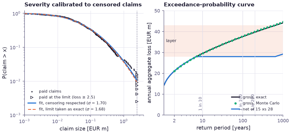
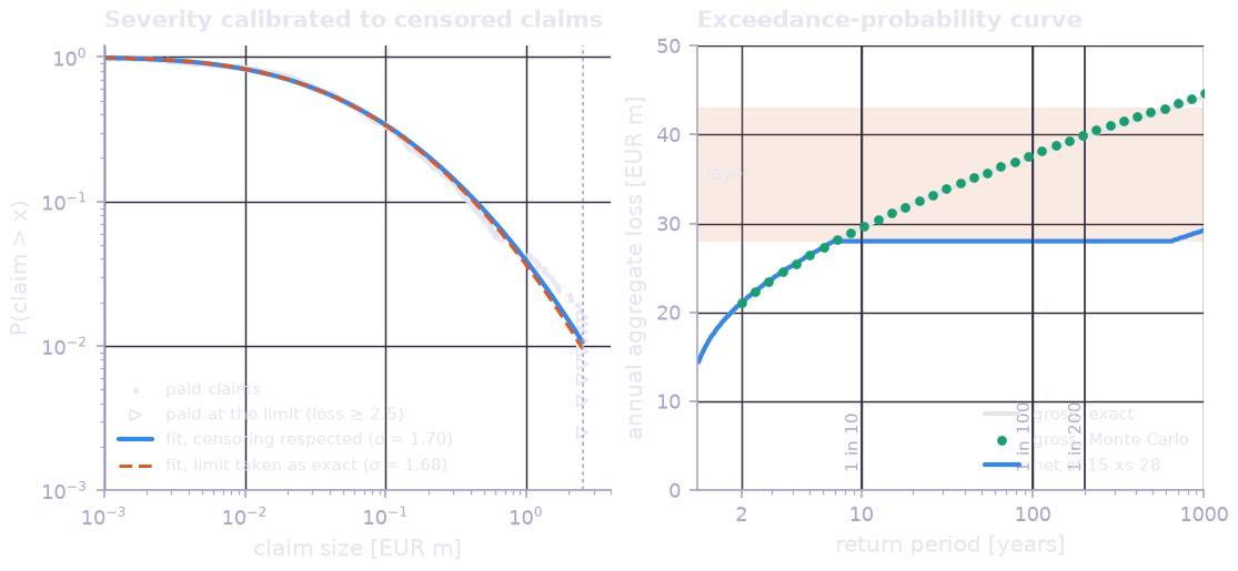
Left: survival function of the paid claims against the fitted log-normal. Treating the ten claims paid at the limit as exact losses thins the fitted tail; with only ten censored claims the difference is small here, but it grows with the share of claims that reach the limit. Right: exceedance- probability curve, the annual loss exceeded once in a given number of years, gross (exact line, Monte Carlo dots) and net of the optimal layer. The treaty caps the retained loss at 28 million up to about the 1-in-650 year level.

Step 5 — Monte Carlo and dependence between lines

The Monte Carlo simulation draws the negative binomial count as a Poisson count with a Gamma-distributed rate, and the claims from the continuous fitted log-normal. It agrees with the exact result to within its sampling error, but needs about 100 000 simulated years to pin down the 99 % tail value-at-risk to 1 %. Panjer’s recursion gives it in a single pass.

A second line, general liability (Poisson 25 claims a year, median claim EUR 80 000, log-sd 1.8), is coupled to the property line through a Gaussian copula on the ranks of their annual losses. The copula samples uniforms, and the exact aggregate quantiles of each line turn them into losses:

copula = prp.GaussianCopula([prp.Uniform(0.0, 1.0), prp.Uniform(0.0, 1.0)], corr_raw=jnp.array([np.arctanh(rho)]))
u = np.asarray(copula.sample(jax.random.PRNGKey(seed), (n_years,)).evaluate({}))
loss_a = AGGREGATE[np.minimum(np.searchsorted(np.cumsum(pmf_a), u[:, 0]), N_AGGREGATE - 1)]
loss_b = AGGREGATE[np.minimum(np.searchsorted(np.cumsum(pmf_b), u[:, 1]), N_AGGREGATE - 1)]

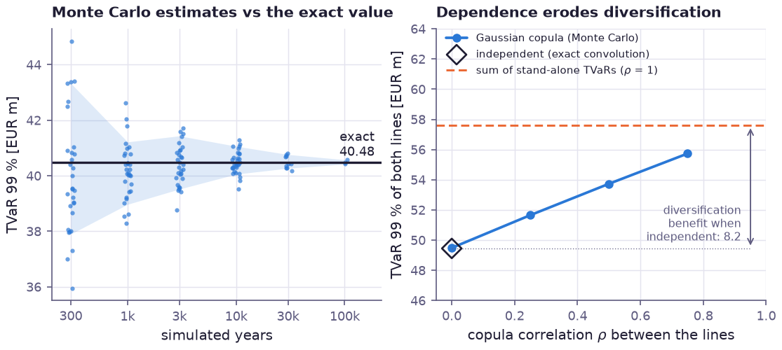
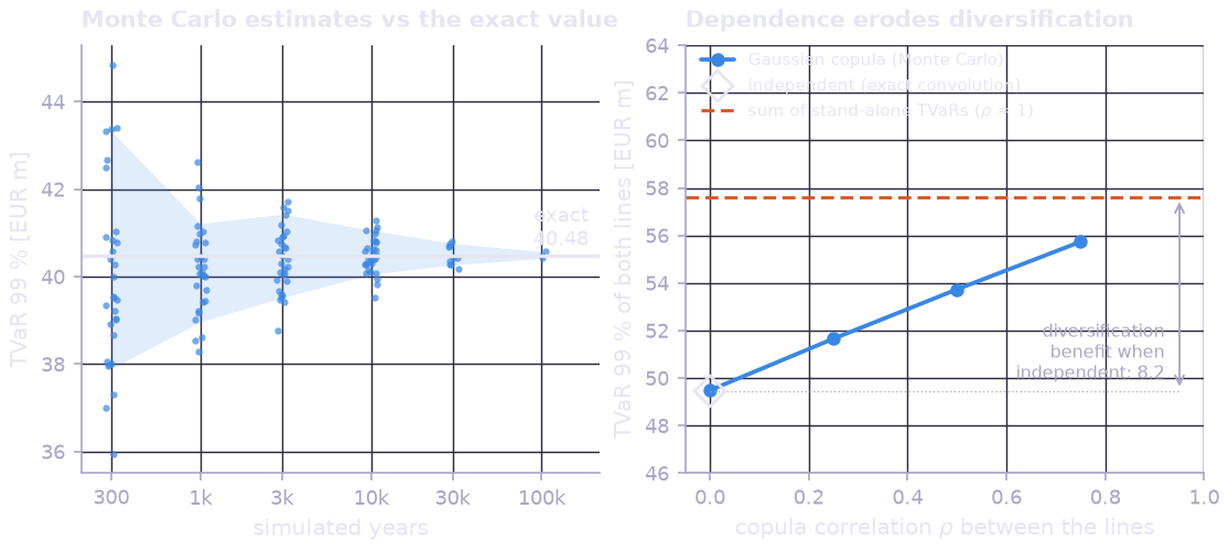
Left: Monte Carlo estimates of the 99 % tail value-at-risk from independent batches of simulated years (dots, 10–90 % band) against the exact value (line). With 1 000 years the estimate can be off by 2 million. Right: the 99 % tail value-at-risk of both lines together. For independent lines, the exact convolution of the two pmfs (diamond) and the copula simulation at zero correlation agree, and pooling saves 8.2 million of capital compared with holding each line on its own. The saving shrinks steadily as the correlation grows, and disappears in the comonotone limit, where tail value-at-risk is additive.

Results

The console output of python examples/insurance_layers/model.py:

=== Severity calibration (600 claims, 10 at the policy limit) ===
  median claim 49.3 kEUR (true 50.0)   log-sd 1.704 (true 1.700)
  ignoring the censoring: log-sd 1.678

=== Annual aggregate loss (Panjer, exact on the lattice) ===
  mass on the lattice 0.999999
  E[S] = 21.51   VaR99.5 = 39.67   TVaR99 = 40.48   [EUR m]

=== Stop-loss 15 xs 20 ===
  expected layer loss 3.115, premium 4.672, capital 7.08 (gross 18.97), total cost 2.266  [EUR m]
  d/dattachment : premium -0.820   capital -0.547
  d/dlimit      : premium +0.034   capital -0.978
  d/dsigma      : premium +21.948   capital +34.869

=== Optimal retention ===
  attachment 27.99 EUR m, P(S > A) = 0.142 (unlimited-layer rule c / (theta + c) = 0.167)
  premium 0.809, capital 7.42, total cost 1.012 (no treaty: 1.897)  [EUR m]

=== Monte Carlo, 100 000 simulated years ===
  E[S] = 21.54   VaR99.5 = 40.02   TVaR99 = 40.80   [EUR m]

=== Property + liability, TVaR99 [EUR m] ===
  stand-alone sum 57.61   independent (exact) 49.45
  Gaussian copula: rho=0.00: 49.49   rho=0.25: 51.66   rho=0.50: 53.74   rho=0.75: 55.74

Primitives exercised

Feature	Used for
Observations, calibrate()	Severity fit with claims capped at the policy limit as right-censored data
LogNormal cdf	Differentiable discretisation of the claim-size distribution
compound_distribution()	Exact aggregate loss pmf, negative binomial and Poisson counts
jax.grad, optimize()	Premium and capital sensitivities; optimal attachment
GaussianCopula	Dependence between the property and liability lines

Running it

$ python examples/insurance_layers/model.py

The run takes about ten seconds on a laptop CPU. The figures on this page are produced by docs/generate_example_insurance_layers.py.